
Three-Term Recurrence Relations and Bessel Functions
Three-term recurrence relations are the basis for computing Bessel functions.
Contents
A Familiar Three-Term Recurrence
Start with two large integers, say 514229 and 317811. For reasons that will soon become clear, I'll label them $f_{30}$ and $f_{29}$.clear n = 30 f(30) = 514229; f(29) = 317811
n =
    30
f =
  Columns 1 through 6
           0           0           0           0           0           0
  Columns 7 through 12
           0           0           0           0           0           0
  Columns 13 through 18
           0           0           0           0           0           0
  Columns 19 through 24
           0           0           0           0           0           0
  Columns 25 through 30
           0           0           0           0      317811      514229
Now take repeated differences, and count backwards.
$$ f_{n-1} = f_{n+1} - f_n, \ n = 29, 28, ..., 2, 1 $$
   for n = 29:-1:2
       f(n-1) = f(n+1) - f(n);
   end
   n
   f
n =
     2
f =
  Columns 1 through 6
           0           1           1           2           3           5
  Columns 7 through 12
           8          13          21          34          55          89
  Columns 13 through 18
         144         233         377         610         987        1597
  Columns 19 through 24
        2584        4181        6765       10946       17711       28657
  Columns 25 through 30
       46368       75025      121393      196418      317811      514229
Recognize those integers? They're the venerable Fibonacci numbers. I've just reversed the usual procedure for computing them. And, I didn't pick the first two values at random. In fact, their choice is very delicate. Try picking any other six-digit integers, and see if you can take 30 differences before you hit a negative value. Of course, we usually start with $f_0 = 0$, $f_1 = 1$ and go forward with additions.
The relation
$$ f_n = f_{n+1} - f_{n-1} $$
is an example of a three-term recurrence. I've written it in such a way that I can go either forward or backward.
Friedrich Bessel
Friedrich Bessel was a German astronomer, mathematician and physicist who lived from 1784 until 1846. He was a contemporary of Gauss, but the two had some sort of falling out. Although he did not have a university education, he made major contributions to precise measurements of planetary orbits and distances to stars. He has a crater on the Moon and an asteroid named after him. In mathematics, the special functions that bear his name were actually discovered by someone else, Daniel Bernoulli, and christened after Bessel's death. They play the same role in polar coordinates that the trig functions play in Cartesian coordinates. They are applicable in a wide range of fields, from physics to finance.Bessel Functions
Bessel functions are defined by an ordinary differential equation that generalizes the harmonic oscillator to polar coordinates. The equation contains a parameter $n$, the order. $$ x^2 y'' + x y' + (x^2 - n^2) y = 0 $$ Solutions to this equation are also sometimes called cylindrical harmonics. For my purposes here, their most important property is the three-term recurrence relation: $$ \frac{2n}{x} J_n(x) = J_{n-1}(x) + J_{n+1}(x) $$ This has a variable coefficient that depends upon the two parameters, the order $n$ and the argument $x$. To complete the specification, it would be necessary to supply two initial conditions that depend upon $x$. But, as we shall see, using the recurrence in the forward direction is disastrous numerically. Alternatively, if we could somehow supply two end conditions, we could use the recurrence in the reverse direction. This the idea behind a classical method known as Miller's algorithm.Miller's Algorithm
Miller's algorithm also employs this interesting identity, which I'll call the normalizer. $$ J_0(x) + 2 J_2(x) + 2 J_4(x) + 2 J_6(x) + \ ... = 1 $$ It's not obvious where this identity comes from and I won't try to derive it here. We don't know the end conditions, but we can pick arbitrary values, run the recurrence backwards, and then use the normalizer to rescale. Step 1. Pick a large $N$ and temporarily let $$ \tilde{J}_N = 0 $$ $$ \tilde{J}_{N-1} = 1 $$ Then for $n = N-1, ..., 1$ compute $$ \tilde{J}_{n-1} = 2n/x \tilde{J}_n \ - \tilde{J}_{n+1} $$ Step 2. Normalize: $$ \sigma = \tilde{J}_0 + 2 \tilde{J}_2 + 2 \tilde{J}_4 + ... $$ $$ J_n = \tilde{J}_n/\sigma, \ n = 0, ..., N $$ I'll show some results in a moment, after I introduce an alternative formulation.Matrix Formulation
You know that I like to describe algorithms in matrix terms. The three-term recurrence generates a tridiagonal matrix. But which three diagonals? I can put the three below the diagonal, above the diagonal, or centered on the diagonal. This is accomplished with the second argument of the sparse matrix generator, spdiags. Here is the code. type blt
function B = blt(n,x,loc)
% BesseL Three term recurence.
% B = blt(n,x,loc) is an n-by-n sparse tridiagonal coefficent matrix
% that generates the Bessel functions besselj((0:n-1)',x).
% loc specifies the location of the diagonals.
%   loc = 'center', the default, centers the three diagonals.
%   loc = 'lower' puts the three diagonals in the lower triangle.
%   loc = 'upper' puts the three diagonals in the upper triangle.

   if nargin == 2
       loc = 'center';
   end

   switch loc
       case 'center', locd = -1:1;
       case 'lower', locd = -2:0;
       case 'upper', locd = 0:2;
   end

   % Three term recurrence: 2*n/x * J_n(x) = J_(n-1)(x) + J_n+1(x).
   d = -2*(0:n-1)'/x;
   e = ones(n,1);
   B = spdiags([e d e],locd,n,n);
end
Lower
If there were no roundoff error, and if we knew the values of the first two Bessel functions, $J_0(x)$ and $J_1(x)$, we could use backslash, the linear equation solver, with the diagonals in the lower triangle to compute $J_n(x)$ for $n > 1$. Here, for example, is $x = 1$.format long J = @(n,x) besselj(n,x); n = 8 x = 1.0 B = blt(n,x,'lower'); rhs = zeros(n,1); rhs(1:2) = J((0:1)',x); v = B\rhs
n =
     8
x =
     1
v =
   0.765197686557967
   0.440050585744934
   0.114903484931901
   0.019563353982668
   0.002476638964110
   0.000249757730213
   0.000020938338022
   0.000001502326053
These values are accurate to almost all the digits shown. Except for the last one. It's beginning to show the effects of severe numerical instability. Let's try a larger value of n.
   n = 18
   B = blt(n,x,'lower');
   rhs = zeros(n,1);
   rhs(1:2) = J((0:1)',x);
   v = B\rhs;
   semilogy(0:n-1,v,'o-')
   title('J_n(1)')
   xlabel('n')
n =
    18
 The values beyond about n = 9 are suspect and, in fact, totally wrong. The forward elimination that backslash uses to solve this lower triangular system is just the three-term recurrence for increasing n. And that recurrence has two solutions -- the one we're trying to compute and a second one corresponding to $Y_n(x)$, the Bessel function of second kind. $Y_n(x)$ is stimulated by roundoff error and completely takes over for $n > 9$.
So the lower triangular option -- the forward recurrence -- is unsatisfactory for two reasons: it requires two Bessel values to get started and it is unstable.
The values beyond about n = 9 are suspect and, in fact, totally wrong. The forward elimination that backslash uses to solve this lower triangular system is just the three-term recurrence for increasing n. And that recurrence has two solutions -- the one we're trying to compute and a second one corresponding to $Y_n(x)$, the Bessel function of second kind. $Y_n(x)$ is stimulated by roundoff error and completely takes over for $n > 9$.
So the lower triangular option -- the forward recurrence -- is unsatisfactory for two reasons: it requires two Bessel values to get started and it is unstable.
Upper
We need to make one modification to the upper triangular coefficient matrix. n = 30;
B = blt(n,x,'upper');
B(n-1,n) = 0;
Now the last two rows and columns are a 2-by-2 identity.
full(B(n-1:n,n-1:n))
ans =
     1     0
     0     1
The back substitution process just runs the three-term recursion backwards. We need to start with $J_{n-1}(x)$ and $J_{n-2}(x)$.
   rhs = zeros(n,1);
   rhs(n-1:n) = J((n-2:n-1)',x);
   format long e
   v = B\rhs
v =
     7.651976865579656e-01
     4.400505857449330e-01
     1.149034849319004e-01
     1.956335398266838e-02
     2.476638964109952e-03
     2.497577302112342e-04
     2.093833800238925e-05
     1.502325817436807e-06
     9.422344172604491e-08
     5.249250179911870e-09
     2.630615123687451e-10
     1.198006746303136e-11
     4.999718179448401e-13
     1.925616764480172e-14
     6.885408200044221e-16
     2.297531532210343e-17
     7.186396586807488e-19
     2.115375568053260e-20
     5.880344573595754e-22
     1.548478441211652e-23
     3.873503008524655e-25
     9.227621982096665e-27
     2.098223955943776e-28
     4.563424055950103e-30
     9.511097932712488e-32
     1.902951751891381e-33
     3.660826744416801e-35
     6.781552053554108e-37
     1.211364502417112e-38
     2.089159981718163e-40
These values are accurate to almost all the significant digits shown. The backwards recursion suppresses the unwanted $Y_n(x)$ and the process is stable.
Center
Can we avoid having to know those two starting values? Yes, by using a matrix formulation of the Miller algorithm. Insert the normalization condition in the first row. Now $B$ is tridiagonal, except for first row, which is[1 0 2 0 2 0 2 ... ]Other rows have $1$ s on the super- and subdiagonal and $-2n/x$ on the diagonal of the $(n+1)$ -st row.
   n = 30;
   B = blt(n,x);
   B(1,1:2) = [1 0];
   B(1,3:2:n) = 2;
   spy(B)
   title('B')
 The beauty of this approach is that it does not require any values of the Bessel function a priori. The right hand side is simply a unit vector.
   rhs = eye(n,1);
   format long e
   v = B\rhs
   semilogy(0:n-1,v,'o-')
   xlabel('n')
   title('J_n(1)')
v =
     7.651976865579665e-01
     4.400505857449335e-01
     1.149034849319005e-01
     1.956335398266840e-02
     2.476638964109954e-03
     2.497577302112343e-04
     2.093833800238926e-05
     1.502325817436807e-06
     9.422344172604494e-08
     5.249250179911872e-09
     2.630615123687451e-10
     1.198006746303136e-11
     4.999718179448401e-13
     1.925616764480171e-14
     6.885408200044220e-16
     2.297531532210343e-17
     7.186396586807487e-19
     2.115375568053260e-20
     5.880344573595753e-22
     1.548478441211652e-23
     3.873503008524655e-25
     9.227621982096663e-27
     2.098223955943775e-28
     4.563424055950102e-30
     9.511097932712487e-32
     1.902951751891381e-33
     3.660826744416762e-35
     6.781552053355331e-37
     1.211364395117367e-38
     2.088559301926495e-40

Relative error
   w = J((0:n-1)',x);
   relerr = (v - w)./w;
   semilogy(0:n-1,abs(relerr) + eps*(v==w),'o-')
   xlabel('n')
   title('relative error')
 The relative error deteriorates for the last few values of n. This is not unexpected because we have effectively truncated a semi-infinite matrix.
Triangular Factors
The LU decomposition of $B$ shows no pivoting for this value of $x$, but there is fill-in. The normalization condition is mixing in with the recurrence. [L,U] = lu(B);
spy(L)
title('L')
snapnow
spy(U)
title('U')


Comments
To leave a comment, please click here to sign in to your MathWorks Account or create a new one.