As the degree of an interpolating polynomial increases, does the polynomial converge to the underlying function? The short answer is maybe. I want to describe a visual tool to help you investigate this question yourself.

Contents

Carl Runge

Carl Runge lived from 1856 until 1927. We know his name because he was the first to write about what we now call the Runge-Kutta method for the numerical solution of ordinary differential equations. His paper was published in 1895. Martin Kutta came along six years later. But Runge made many other contributions, including the subject of today's post.

A classical result of Runge's advisor, Karl Weierstrass, is that for any continuous function, there exists a sequence of polynomials of increasing order that converge uniformly to the function. But this result does not tell us whether the polynomials can be interpolating or where the interpolating points might be located.

Runge's famous counterexample for interpolation is the function

$f(x) = \frac{1}{1+25x^2}$

If this function is interpolated at equally spaced points in the interval [-1,1], the polynomials do not converge uniformly. In fact, the maximum error goes to infinity.

interp_gadget

I call my MATLAB® program interp_gadget. You can vary three parameters, $c$, $n$ and $w$. You can choose one of the three target functions involving the coefficient $c$.

$f_1(x) = \frac{1}{1+c x^2}$

$f_2(x) = e^{-c x^2}$

$f_3(x) = |cx|$

The parameter $n$ is the number of interpolation points in the interval [-1 1]. The degree of the interpolating polynomial is $n-1$.

The distribution of the points involves the weight $w$. The points are a weighted average between equally spaced points and Chebyshev points concentrated towards the end of the interval.

$x_{ch} = \cos({\frac{n-\frac{1}{2}:-1:\frac{1}{2}}{n}\pi})$

$x_{eq} = -1:\frac{2}{n-1}:1$

$x = wx_{ch} + (1-w)x_{eq}$

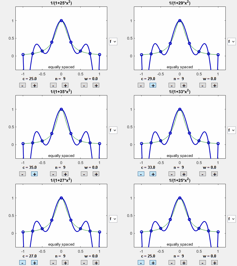
The green curve in the following animations and plots is the target function $f(x)$ and the blue curve is the polynomial that interpolates the target at the blue circles. The interpolation error is the difference between the two curves.

Vary coefficient

Let's vary the coefficient $c$ in the bell-shaped target $f_1$, while keeping the number of equally spaced points fixed. The value $c = 25$ gives us Runge's function. As $c$ increases, the peak in the target becomes sharper and the interpolation error increases.

Vary number of points

Let's vary the number of points, while keeping the target fixed and the points equally spaced. As $n$ increases, we see the error near the ends of the interval increase dramatically.

Vary weight

Let's vary the weight in the point distribution. As we move from equal spacing towards Chebyshev spacing, the error near the end points decreases significantly.

Initial configuration

Now some static plots comparing a few different settings of the parameters. Here is the initial setting with Runge's value of $c$ and nine equally spaced interpolation points.

High degree

Increase the number of points while keeping them equally spaced. There is trouble near the end points.

Chebyshev distribution

Distributing a modest number of points nearer the ends of the interval is a big improvement.

Gaussian target

The Gaussian target $f_2(x)$ behaves pretty much like Runge's.

abs(x)

Behavior with the target $f_3(x)$ warrants further investigation.

Extra credit

Here is Runge's example again, with many equally spaced interpolation points. I've added red lines at $x = \pm .726$. In section 3.4 of a classic numerical analysis text that is now available as an inexpensive Dover reprint, Dover link, Eugene Isaacson and Herb Keller begin a proof of the fact that polynomial interpolation converges for $x$ between these red lines and diverges for $x$ outside them. But a key portion of their proof is left as an exercise.

So, I have a few tasks for those inclined to undertake them. The first is to finish Isaacson and Keller's argument, which explains where the $.726$ comes from. How does $.726$ depend on the coefficient $c$ in function $f_1(x)$? Where are the red lines for our two other target functions? How does their location depend upon $w$?

I don't know the answers to these questions. If you discover something, please let us know in the comments.

Software

I have submitted interp_gadget to the MATLAB Central file exchange, available at this link. It is also included in version 4.01 of Cleve's Laboratory, available at this link.

Get the MATLAB code

Published with MATLAB® R2018b