
Penrose and Fourier Design Playing Cards
MathWorks is creating a deck of playing cards that will be offered as gifts at our trade show booths. The design of the cards is based on Penrose Tilings and plots of the Finite Fourier Transform Matrix.
Contents
Penrose Tilings
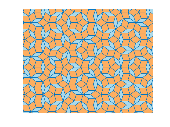
This is an example of a Penrose tiling.

Penrose tilings are aperiodic tilings of the plane named after Oxford emeritus physicist Roger Penrose, who studied them in the 1970s. MathWorks' Steve Eddins has written a paper about his MATLAB program for generating Penrose tilings. I will include the paper in this blog post. Steve has also submitted his paper and code to the MATLAB Central File Exchange, Penrose Rhombus Tiling.
The Suits
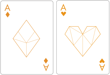
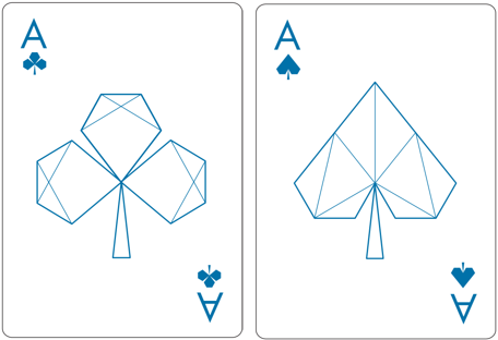
Look carefully at the example tiling. It's made entirely from two rhombuses, one colored gold and one colored blue. Each rhombus, in turn, is made from two isosceles triangles. These shapes inspired MathWorks designer Gabby Lydon to reimagine the traditional symbols for the four suits in a deck of cards.
Here are the diamonds and hearts.
Here are the clubs and spades.
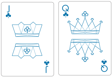
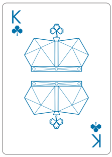
The Face Cards
The theme of triangles and rhombuses is continued in the face cards.
The Back
The backs of the cards feature two mathematical objects that I have described in this blog. I wrote a five-part series about our logo five years ago, beginning with part one. And, I wrote about the graphic produced by the Finite Fourier Transform matrix.
Start with a prime integer.
n = 31;
Take a Fourier transform of the columns of the identity matrix.
F = fft(eye(n,n));
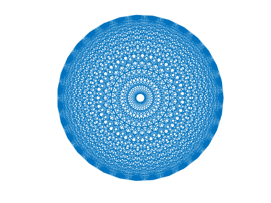
Plot it. Because 31 is prime, this is the complete graph on 31 points. Every point on the circumference is connected to every other point.
   p = plot(F);
   axis square
   axis off
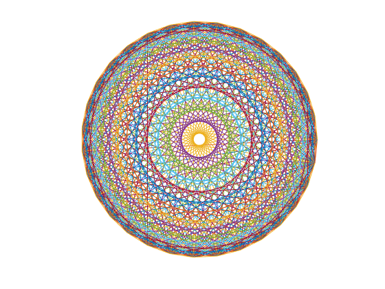
That's too colorful.
   color = get(gca,'colororder');
   set(p,'color',color(1,:))
Now graphic design software takes over and makes room for the logo.

Cleve's Lab
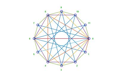
All this has reminded me of two FFT-related apps from Numerical Computing with MATLAB, fftgui and fftmatrix. I've added them to Cleve's Laboratory with Version 3.9. This is the image from fftmatrix for n = 12. Because 12 is not prime, this is not a completely connected graph. You can vary both the matrix order and the columns to be transformed.
Now, here is Steve's paper about Penrose tiling.
Penrose Rhombus Tiling
by Steve Eddins
This story is about creating planar tilings like this:
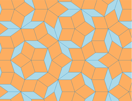
This is an example of a Penrose tiling. Penrose tilings are aperiodic tilings that named after Roger Penrose, who studied them in the 1970s. This particular form, made from two rhombuses, is called a P3 tiling.
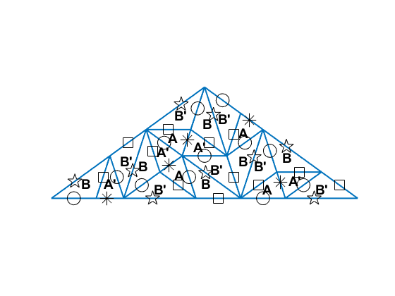
Four Types of Triangles
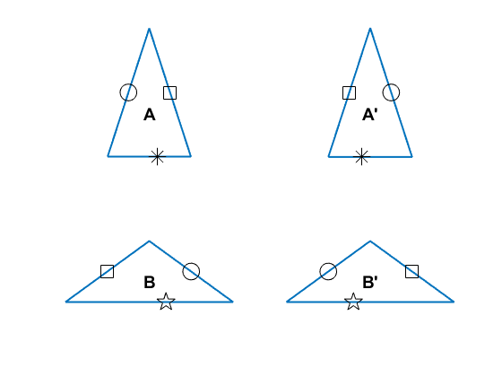
Construction of a Penrose P3 tiling is based on 4 types of isosceles triangles. The types are labeled A, A', B, and B'. The A and A' triangles have an apex angle of 36 degrees, and the B and B' triangles have an apex angle of 72 degrees.
subplot(2,2,1)
showLabeledTriangles(aTriangle([],-1,1))

subplot(2,2,2)
showLabeledTriangles(apTriangle([],-1,1))

subplot(2,2,3)
showLabeledTriangles(bTriangle([],-1,1))

subplot(2,2,4)
showLabeledTriangles(bpTriangle([],-1,1))
vertices =
  -1.0000 + 0.0000i   0.0000 + 3.0777i   1.0000 + 0.0000i
vertices =
  -1.0000 + 0.0000i   0.0000 + 3.0777i   1.0000 + 0.0000i
vertices =
  -1.0000 + 0.0000i   0.0000 + 0.7265i   1.0000 + 0.0000i
vertices =
  -1.0000 + 0.0000i   0.0000 + 0.7265i   1.0000 + 0.0000i
Triangle Functions and Triangle Representation
Before proceeding further, let's pause to look at what the functions aTriangle, apTriangle, bTriangle, and bpTriangle do.
The function aTriangle takes three arguments: aTriangle(apex,left,right). Each of the three arguments is a point in the complex plane that represents one triangle vertex. You specify any two points, passing in the third point as [], and aTriangle computes the missing vertex for you. Here's an example showing how to compute a type A triangle whose base is on the real axis, extending from -1 to 1.
t_a = aTriangle([],-1,1)
t_a =
  1×4 table
      Apex       Left    Right    Type
    _________    ____    _____    ____
    0+3.0777i     -1       1       A
The result is returned as a table, which is convenient because we'll be creating large collections of these triangles, and it is helpful to be able to refer to the different vertices of the triangles using the notation t.Apex, t.Left, and t.Right.
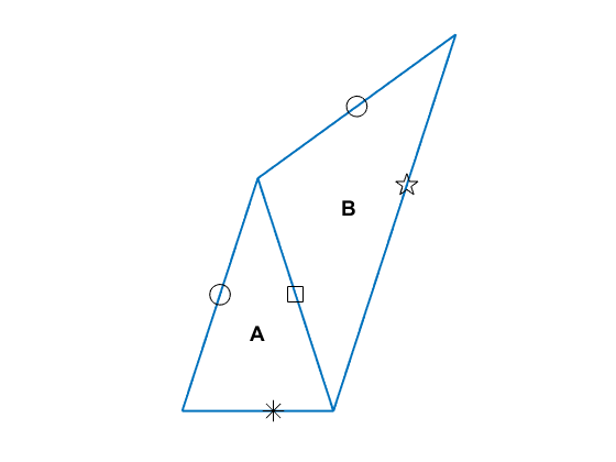
The function showLabeledTriangles takes a table of triangles and displays them all, with the triangle types and their sides labeled. (We'll talk more about the labeling of the sides below.)
t_b = bTriangle(t_a.Apex,t_a.Right,[]);
T = [t_a ; t_b]
clf
showLabeledTriangles(T)
T =
  2×4 table
      Apex       Left        Right        Type
    _________    ____    _____________    ____
    0+3.0777i     -1         1+0i          A
    0+3.0777i      1     2.618+4.9798i     B
vertices =
  -1.0000 + 0.0000i   0.0000 + 3.0777i   1.0000 + 0.0000i
   1.0000 + 0.0000i   0.0000 + 3.0777i   2.6180 + 4.9798i
Triangle Side Labels
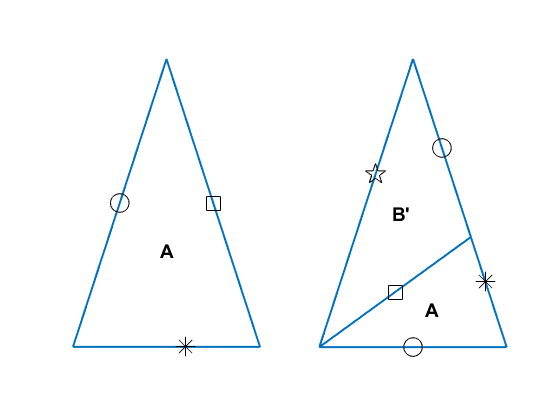
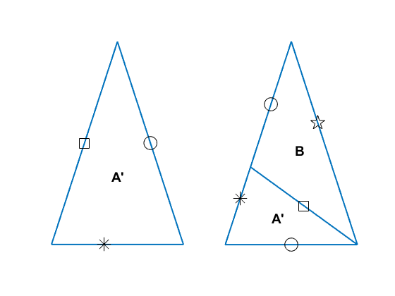
The markers on the sides of the triangles help us to distinguish between A and A' triangles, as well as between B and B' triangles. For example, an A triangle has the circle marker on the left side (assuming the apex is oriented at the top), whereas the A' triangle has the circle marker on the right side.
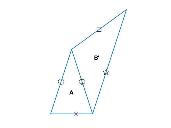
The side labels also help us confirm whether we have a correct arrangement of triangles in our Penrose tiling. Triangles are only allowed to share an edge in the Penrose P3 tiling if the side markers align together and are the same. For example, in the two triangles shown above, the square marker on the right edge of the triangle lines up with the square marker on the left edge of the B triangle. If we had used a B' triangle instead, the markers would not have been identical.
t_bp = bpTriangle(t_a.Apex,t_a.Right,[]);
T = [t_a ; t_bp];
showLabeledTriangles(T)
vertices =
  -1.0000 + 0.0000i   0.0000 + 3.0777i   1.0000 + 0.0000i
   1.0000 + 0.0000i   0.0000 + 3.0777i   2.6180 + 4.9798i
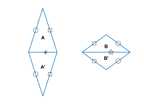
Making the Two Types of Rhombus
In the Penrose P3 tiling, one rhombus is made from an A and an A' triangle, and the other is made from a B and a B' triangle.
subplot(1,2,1)
r1 = [ ...
    aTriangle([],-1,1)
    apTriangle([],1,-1)];
showLabeledTriangles(r1)

subplot(1,2,2)
r2 = [ ...
    bTriangle([],-1,1)
    bpTriangle([],1,-1)];
showLabeledTriangles(r2)
vertices =
  -1.0000 + 0.0000i   0.0000 + 3.0777i   1.0000 + 0.0000i
   1.0000 + 0.0000i   0.0000 - 3.0777i  -1.0000 + 0.0000i
vertices =
  -1.0000 + 0.0000i   0.0000 + 0.7265i   1.0000 + 0.0000i
   1.0000 + 0.0000i   0.0000 - 0.7265i  -1.0000 + 0.0000i
Triangle Decomposition
Construction of the P3 tiling proceeds by starting with one triangle and then successively decomposing it. Each of the four types of triangles has a different rule for decomposition.
An A triangle decomposes into an A triangle and a B' triangle.
t_a = aTriangle([],-1,1);
t_a_d = decomposeATriangle(t_a)

clf
subplot(1,2,1)
showLabeledTriangles(t_a)
lims = axis;
subplot(1,2,2)
showLabeledTriangles(t_a_d)
axis(lims)
t_a_d =
  2×4 table
         Apex            Left            Right         Type
    _______________    _________    _______________    ____
         -1+0i         1+0i         0.61803+1.1756i     A
    0.61803+1.1756i    0+3.0777i         -1+0i          Bp
vertices =
  -1.0000 + 0.0000i   0.0000 + 3.0777i   1.0000 + 0.0000i
vertices =
   1.0000 + 0.0000i  -1.0000 + 0.0000i   0.6180 + 1.1756i
   0.0000 + 3.0777i   0.6180 + 1.1756i  -1.0000 + 0.0000i
You can look at the very short implementation of decomposeATriangle to see how this is done.
function out = decomposeATriangle(in)
out = [ ...
    aTriangle(in.Left,in.Right,[])
    bpTriangle([],in.Apex,in.Left) ];
The smaller A triangle is determined by placing its apex at the left vertex of the input triangle and placing its left vertex at the right vertex of the input triangle.
The smaller B' triangle is determined by placing its left vertex at the apex of the input triangle and placing its right vertex at the left vertex of the input triangle.
There are similar rules for decomposing the other three types of triangles.
t_ap = apTriangle([],-1,1);
t_ap_d = decomposeApTriangle(t_ap)

clf
subplot(1,2,1)
showLabeledTriangles(t_ap)
lims = axis;
subplot(1,2,2)
showLabeledTriangles(t_ap_d)
axis(lims)
t_ap_d =
  2×4 table
          Apex                Left            Right       Type
    ________________    ________________    __________    ____
           1+0i         -0.61803+1.1756i    -1+0i          Ap
    -0.61803+1.1756i           1+0i          0+3.0777i     B
vertices =
  -1.0000 + 0.0000i   0.0000 + 3.0777i   1.0000 + 0.0000i
vertices =
  -0.6180 + 1.1756i   1.0000 + 0.0000i  -1.0000 + 0.0000i
   1.0000 + 0.0000i  -0.6180 + 1.1756i   0.0000 + 3.0777i
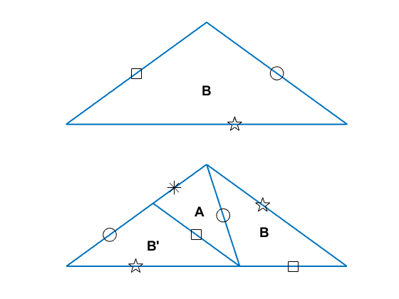
t_b = bTriangle([],-1,1);
t_b_d = decomposeBTriangle(t_b)

clf
subplot(2,1,1)
showLabeledTriangles(t_b)
lims = axis;
subplot(2,1,2)
showLabeledTriangles(t_b_d)
axis(lims)
t_b_d =
  3×4 table
          Apex              Left              Right          Type
    _________________    ___________    _________________    ____
     0.23607+0i           1+0i                 0+0.72654i     B
     0.23607+0i           0+0.72654i    -0.38197+0.44903i     A
    -0.38197+0.44903i    -1+0i           0.23607+0i           Bp
vertices =
  -1.0000 + 0.0000i   0.0000 + 0.7265i   1.0000 + 0.0000i
vertices =
   1.0000 + 0.0000i   0.2361 + 0.0000i   0.0000 + 0.7265i
   0.0000 + 0.7265i   0.2361 + 0.0000i  -0.3820 + 0.4490i
  -1.0000 + 0.0000i  -0.3820 + 0.4490i   0.2361 + 0.0000i
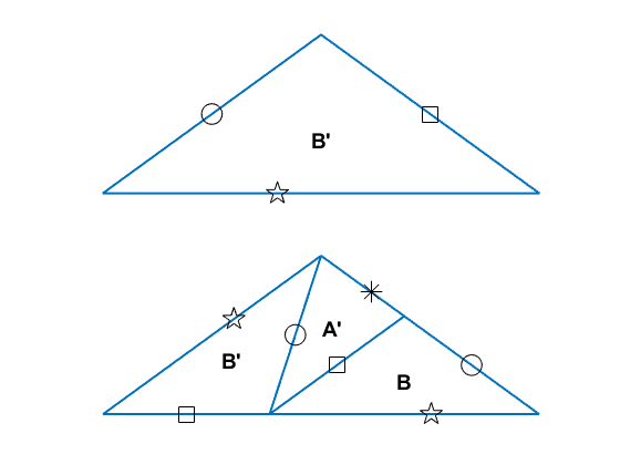
t_bp = bpTriangle([],-1,1);
t_bp_d = decomposeBpTriangle(t_bp)

clf
subplot(2,1,1)
showLabeledTriangles(t_bp)
lims = axis;
subplot(2,1,2)
showLabeledTriangles(t_bp_d)
axis(lims)
t_bp_d =
  3×4 table
          Apex                 Left              Right       Type
    _________________    _________________    ___________    ____
    -0.23607+0i                 0+0.72654i    -1+0i           Bp
    -0.23607+0i           0.38197+0.44903i     0+0.72654i     Ap
     0.38197+0.44903i    -0.23607+0i           1+0i           B
vertices =
  -1.0000 + 0.0000i   0.0000 + 0.7265i   1.0000 + 0.0000i
vertices =
   0.0000 + 0.7265i  -0.2361 + 0.0000i  -1.0000 + 0.0000i
   0.3820 + 0.4490i  -0.2361 + 0.0000i   0.0000 + 0.7265i
  -0.2361 + 0.0000i   0.3820 + 0.4490i   1.0000 + 0.0000i
From Triangles to Rhombuses
Let's start with a B triangle and decompose it three times successively.
t = bTriangle([],-1,1);
t = decomposeTriangles(t)
t = decomposeTriangles(t)
t = decomposeTriangles(t)
t =
  3×4 table
          Apex              Left              Right          Type
    _________________    ___________    _________________    ____
     0.23607+0i           1+0i                 0+0.72654i     B
     0.23607+0i           0+0.72654i    -0.38197+0.44903i     A
    -0.38197+0.44903i    -1+0i           0.23607+0i           Bp
t =
  8×4 table
          Apex                 Left                 Right          Type
    _________________    _________________    _________________    ____
     0.38197+0.44903i           0+0.72654i     0.23607+0i           B
     0.38197+0.44903i     0.23607+0i           0.52786+0i           A
     0.52786+0i                 1+0i           0.38197+0.44903i     Bp
           0+0.72654i    -0.38197+0.44903i     -0.1459+0.27751i     A
     -0.1459+0.27751i     0.23607+0i                 0+0.72654i     Bp
    -0.52786+0i          -0.38197+0.44903i          -1+0i           Bp
    -0.52786+0i           -0.1459+0.27751i    -0.38197+0.44903i     Ap
     -0.1459+0.27751i    -0.52786+0i           0.23607+0i           B
t =
  21×4 table
           Apex                 Left                 Right           Type
    __________________    _________________    __________________    ____
       0.1459+0.27751i     0.23607+0i            0.38197+0.44903i     B
       0.1459+0.27751i     0.38197+0.44903i      0.23607+0.55503i     A
      0.23607+0.55503i           0+0.72654i       0.1459+0.27751i     Bp
      0.23607+0i           0.52786+0i            0.47214+0.17151i     A
      0.47214+0.17151i     0.38197+0.44903i      0.23607+0i           Bp
      0.76393+0.17151i     0.52786+0i                  1+0i           Bp
      0.76393+0.17151i     0.47214+0.17151i      0.52786+0i           Ap
      0.47214+0.17151i     0.76393+0.17151i      0.38197+0.44903i     B
     -0.38197+0.44903i     -0.1459+0.27751i     -0.09017+0.44903i     A
     -0.09017+0.44903i           0+0.72654i     -0.38197+0.44903i     Bp
       0.1459+0.27751i     -0.1459+0.27751i      0.23607+0i           Bp
       0.1459+0.27751i    -0.09017+0.44903i      -0.1459+0.27751i     Ap
     -0.09017+0.44903i      0.1459+0.27751i            0+0.72654i     B
     -0.61803+0.27751i    -0.52786+0i           -0.38197+0.44903i     Bp
     -0.61803+0.27751i     -0.7082+0i           -0.52786+0i           Ap
      -0.7082+0i          -0.61803+0.27751i           -1+0i           B
     -0.38197+0.44903i     -0.2918+0.17151i      -0.1459+0.27751i     Ap
      -0.2918+0.17151i    -0.38197+0.44903i     -0.52786+0i           B
    -0.055728+0i           0.23607+0i            -0.1459+0.27751i     B
    -0.055728+0i           -0.1459+0.27751i      -0.2918+0.17151i     A
      -0.2918+0.17151i    -0.52786+0i          -0.055728+0i           Bp
clf
showLabeledTriangles(t)
vertices =
   0.2361 + 0.0000i   0.1459 + 0.2775i   0.3820 + 0.4490i
   0.3820 + 0.4490i   0.1459 + 0.2775i   0.2361 + 0.5550i
   0.0000 + 0.7265i   0.2361 + 0.5550i   0.1459 + 0.2775i
   0.5279 + 0.0000i   0.2361 + 0.0000i   0.4721 + 0.1715i
   0.3820 + 0.4490i   0.4721 + 0.1715i   0.2361 + 0.0000i
   0.5279 + 0.0000i   0.7639 + 0.1715i   1.0000 + 0.0000i
   0.4721 + 0.1715i   0.7639 + 0.1715i   0.5279 + 0.0000i
   0.7639 + 0.1715i   0.4721 + 0.1715i   0.3820 + 0.4490i
  -0.1459 + 0.2775i  -0.3820 + 0.4490i  -0.0902 + 0.4490i
   0.0000 + 0.7265i  -0.0902 + 0.4490i  -0.3820 + 0.4490i
  -0.1459 + 0.2775i   0.1459 + 0.2775i   0.2361 + 0.0000i
  -0.0902 + 0.4490i   0.1459 + 0.2775i  -0.1459 + 0.2775i
   0.1459 + 0.2775i  -0.0902 + 0.4490i   0.0000 + 0.7265i
  -0.5279 + 0.0000i  -0.6180 + 0.2775i  -0.3820 + 0.4490i
  -0.7082 + 0.0000i  -0.6180 + 0.2775i  -0.5279 + 0.0000i
  -0.6180 + 0.2775i  -0.7082 + 0.0000i  -1.0000 + 0.0000i
  -0.2918 + 0.1715i  -0.3820 + 0.4490i  -0.1459 + 0.2775i
  -0.3820 + 0.4490i  -0.2918 + 0.1715i  -0.5279 + 0.0000i
   0.2361 + 0.0000i  -0.0557 + 0.0000i  -0.1459 + 0.2775i
  -0.1459 + 0.2775i  -0.0557 + 0.0000i  -0.2918 + 0.1715i
  -0.5279 + 0.0000i  -0.2918 + 0.1715i  -0.0557 + 0.0000i
Now the labels are getting in the way.
showTriangles(t)
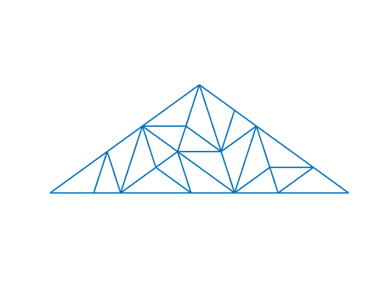
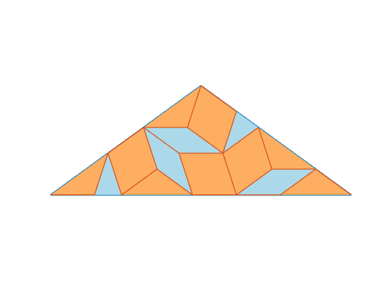
That's better, but it's hard to visualize the rhombuses because the triangle bases are being drawn. Let's switch to a different visualization function that draws the rhombuses with colored shading and without the triangle bases.
showTiles(t)
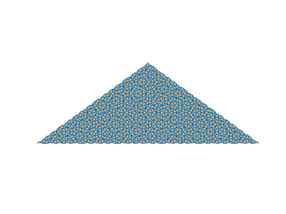
Let's do five more levels of decomposition.
for k = 1:5
    t = decomposeTriangles(t);
end

num_triangles = height(t)
num_triangles =
        2584
Now we have lots of triangles. Let's take a look.
clf
showTiles(t)
Zoom in.
axis([-0.3 0.2 0.1 0.5])
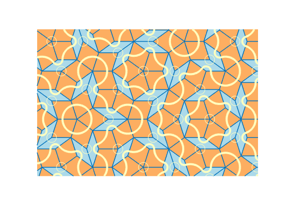
For fun, you can add to the visualization by inserting arcs or other shapes in the triangles. You just need to make everything match up across the different types of triangles. The showDecoratedTiles function shows one possible variation.
clf
showDecoratedTiles(t)
axis([-0.2 0.1 0.2 0.4])
Starting from Multiple Triangles
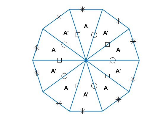
Another interesting thing to try is to start from a pattern of multiple triangles instead of just one. You just to arrange the initial triangles so that they satisfy the side matching rules. Let's use a circular pattern of alternating A and A' triangles sharing a common apex.
t = table;
for k = 1:5
    thetad = 72*(k-1);
    t_a = aTriangle(0,cosd(thetad) + 1i*sind(thetad),[]);
    t_ap = apTriangle(0,t_a.Right,[]);
    t = [t ; t_a ; t_ap];
end
showLabeledTriangles(t)
vertices =
   1.0000 + 0.0000i   0.0000 + 0.0000i   0.8090 + 0.5878i
   0.8090 + 0.5878i   0.0000 + 0.0000i   0.3090 + 0.9511i
   0.3090 + 0.9511i   0.0000 + 0.0000i  -0.3090 + 0.9511i
  -0.3090 + 0.9511i   0.0000 + 0.0000i  -0.8090 + 0.5878i
  -0.8090 + 0.5878i   0.0000 + 0.0000i  -1.0000 + 0.0000i
  -1.0000 + 0.0000i   0.0000 + 0.0000i  -0.8090 - 0.5878i
  -0.8090 - 0.5878i   0.0000 + 0.0000i  -0.3090 - 0.9511i
  -0.3090 - 0.9511i   0.0000 + 0.0000i   0.3090 - 0.9511i
   0.3090 - 0.9511i   0.0000 + 0.0000i   0.8090 - 0.5878i
   0.8090 - 0.5878i   0.0000 + 0.0000i   1.0000 + 0.0000i
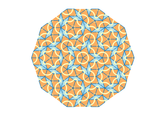
t2 = t;
for k = 1:4
    t2 = decomposeTriangles(t2);
end
clf
showDecoratedTiles(t2)


Comments
To leave a comment, please click here to sign in to your MathWorks Account or create a new one.