
Round, With Ties to Even
We are considering a MATLAB Enhancement Request to support options for round(x) when x is exactly halfway between two integers.
Contents
Classic round
The Classic MATLAB calculator was written in Fortran forty years ago, before IEEE 754 and before MathWorks. It had only 71 functions and it was not easy to add more. But one of those functions was ROUND. The help entry had only one sentence.
ROUND ROUND(X) rounds the elements of X to the nearest integers.
That doesn't say what happens when there is a tie. The code for ROUND was essentially this one line, which relied on FLOOR.
ROUND(X) = SIGN(X)*FLOOR(ABS(X) + 0.5)
In particular:
ROUND(0.5) = 1.0
ROUND(1.5) = 2.0.
When MathWorks began producing the modern versions of MATLAB in 1984, we retained this simple definition for round.
roundoff
The function round can be used to clean up after roundoff.
   format long e
   H = hilb(5)
   X = inv(H)
   X = round(X)
   XH = X*H
   XH = round(XH)
H =

  Columns 1 through 3

     1.000000000000000e+00     5.000000000000000e-01     3.333333333333333e-01
     5.000000000000000e-01     3.333333333333333e-01     2.500000000000000e-01
     3.333333333333333e-01     2.500000000000000e-01     2.000000000000000e-01
     2.500000000000000e-01     2.000000000000000e-01     1.666666666666667e-01
     2.000000000000000e-01     1.666666666666667e-01     1.428571428571428e-01

  Columns 4 through 5

     2.500000000000000e-01     2.000000000000000e-01
     2.000000000000000e-01     1.666666666666667e-01
     1.666666666666667e-01     1.428571428571428e-01
     1.428571428571428e-01     1.250000000000000e-01
     1.250000000000000e-01     1.111111111111111e-01


X =

  Columns 1 through 3

     2.499999999998526e+01    -2.999999999997500e+02     1.049999999998995e+03
    -2.999999999997500e+02     4.799999999995864e+03    -1.889999999998367e+04
     1.049999999998995e+03    -1.889999999998367e+04     7.937999999993641e+04
    -1.399999999998561e+03     2.687999999997693e+04    -1.175999999999111e+05
     6.299999999993241e+02    -1.259999999998929e+04     5.669999999995910e+04

  Columns 4 through 5

    -1.399999999998561e+03     6.299999999993241e+02
     2.687999999997693e+04    -1.259999999998929e+04
    -1.175999999999111e+05     5.669999999995910e+04
     1.791999999998769e+05    -8.819999999994377e+04
    -8.819999999994377e+04     4.409999999997448e+04


X =

          25        -300        1050       -1400         630
        -300        4800      -18900       26880      -12600
        1050      -18900       79380     -117600       56700
       -1400       26880     -117600      179200      -88200
         630      -12600       56700      -88200       44100


XH =

  Columns 1 through 3

     1.000000000000000e+00                         0                         0
                         0     1.000000000000000e+00                         0
                         0                         0     1.000000000000000e+00
                         0                         0    -3.637978807091713e-12
                         0                         0                         0

  Columns 4 through 5

                         0                         0
                         0                         0
                         0                         0
     1.000000000000000e+00                         0
                         0     1.000000000000000e+00


XH =

     1     0     0     0     0
     0     1     0     0     0
     0     0     1     0     0
     0     0     0     1     0
     0     0     0     0     1
flints
round works on an array element-wise, mapping all elements to flints, floating point numbers whose values are integers. All values less than one-half are mapped to zero. All values larger than flintmax are already flints, so they are mapped to themselves. And all values between one-half and flintmax, except those exactly halfway between two flints, are mapped to the nearest flints. Pretty much everybody agrees to all of that.
The only leeway, and the primary reason for the Enhancement Request and this blog post, is the behavior of round for values exactly halfway between two flints.
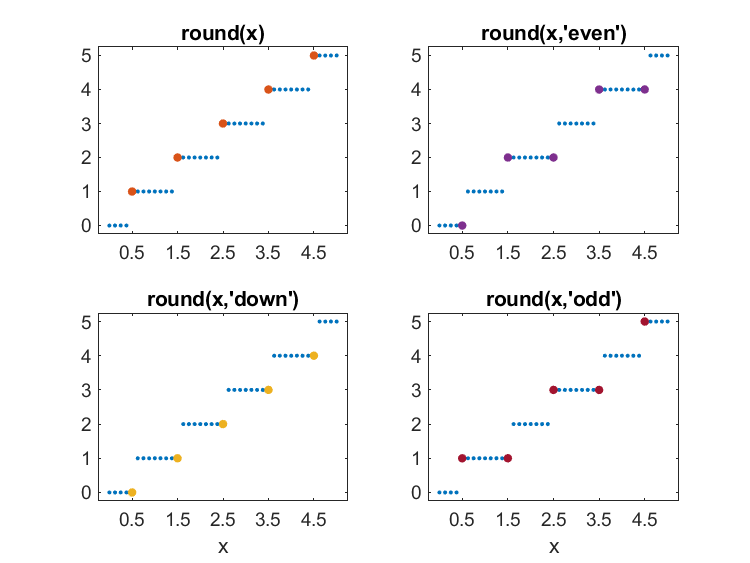
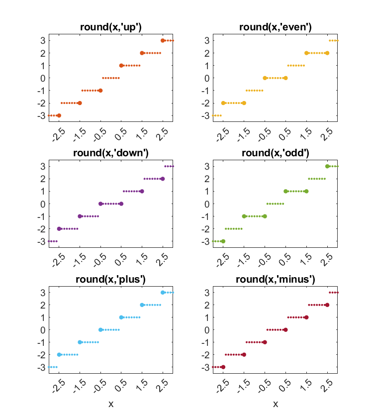
round
I suggest that we add a tie-breaker option to the built-in function round. If you don't use this ties option, round will continue to function as it always has. And if you never encounter a tie, all of these options give the same results.
The most important option is 'even'. There is a statistical argument to be made in its favor. If you never encounter a tie, the mean of expected changes made by rounding data is zero. With the 'even' option', that is still true even if you do encounter ties.
The 'up' option is the default and the traditional MATLAB behavior. The 'odd' and 'down' options together provide a mirror image of the 'even' and 'up' pair.
type Round
function r = round(x,ties)
% r = round(x) rounds the elements of x to the nearest integers.
% Elements halfway between integers are rounded away from zero.
%
% r = round(x,'even') rounds to integers, ties to even.
% r = round(x,'odd') rounds to integers, ties to odd.
% r = round(x,'down') rounds to integers, ties towards zero.
% r = round(x,'up') rounds to integers, ties away from zero (default).
%
   a = abs(x) + 0.5;
   r = floor(a);
   if nargin == 2
       switch ties
           case 'even'
               m = (r == a) & (mod(r,2) == 1);
           case 'odd'
               m = (r == a) & (mod(r,2) == 0);
           case 'down'
               m = (r == a);
           case 'up'
               m = [];
       end
       r(m) = r(m) - 1;
   end
   r = sign(x).*r;
end
test round
   x = (0.5:1:4.5)';
   xRound(x)
     x    round  even  down   odd

   0.500     1     0     0     1
   1.500     2     2     1     1
   2.500     3     2     2     3
   3.500     4     4     3     3
   4.500     5     4     4     5
cities
Download the spread sheet available at www.census.gov/cities and use the Import Wizard to select the last column. This gives us the population of 788 US cities in 2019.
load cities.mat cities census
Round the data to nearest 1,000.
rcensus = 1000*Round(census/1000);
Here are the five largest cities, their population, and that population rounded.
    disp(cities(1:5))
    disp([census(1:5) rcensus(1:5)])
    "New York city, New York"
    "Los Angeles city, California"
    "Chicago city, Illinois"
    "Houston city, Texas"
    "Phoenix city, Arizona"

     8336817     8337000
     3979576     3980000
     2693976     2694000
     2320268     2320000
     1680992     1681000
And here are the five smallest,
    disp(cities(end-4:end))
    disp([census(end-4:end) rcensus(end-4:end)])
    "Lakewood city, Ohio"
    "Troy city, New York"
    "Saginaw city, Michigan"
    "Niagara Falls city, New York"
    "Charleston city, West Virginia"

       49678       50000
       49154       49000
       48115       48000
       47720       48000
       46536       47000
Here is the histogram of the changes made by rounding. Despite its ragged appearance, this is uniform.
    delta = census - rcensus;
    histogram(delta,40)
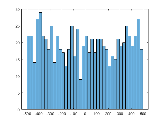
About half of the 788 rounded down and about half rounded up. Only one city reported a 2019 population that was already a multiple of 1,000.
disp([nnz(delta < 0), nnz(delta == 0), nnz(delta > 0)])
396 1 391
   k = find(delta == 0)
   disp(cities(k))
   disp([census(k) rcensus(k)])
k =

    69

Anchorage municipality, Alaska
      288000      288000
How many cities reported population ties, i.e. populations halfway between multiples of 1,000?
   k = find(mod(census,1000)==500)
   disp(cities(k))
   disp([census(k) rcensus(k)])
k =

   131
   189
   757

    "Tallahassee city, Florida"
    "Roseville city, California"
    "Burien city, Washington"

      194500      195000
      141500      142000
       51500       52000
Only one city out of the 788 reported a tie and a population that rounded to an odd multiple of 1,000, there by triggering the 'even' option.
   ecensus = 1000*Round(census/1000,'even');
   k = find(ecensus ~= rcensus)
   disp(cities(k))
   disp([census(k) rcensus(k)  ecensus(k)])
k =

   131

Tallahassee city, Florida
      194500      195000      194000
IEEE 754
The IEEE 754 rounding modes are easily confused with the round function. IEEE 754 is about hardware; round is software. Floating point arithmetic operations are taking place at an accuracy scale that is 16 orders of magnitude finer and at a rate that is many orders of magnitude faster. Some of the considerations are similar, but the setting and the details are very different.
Which?
Should MATLAB have something like round(x,'even')? It's really a matter of taste. I happen to like the way we've always done things. To others, the statistical properties of round-ties-to-even might be relevant.
But I think the most important argument in favor of the Enhancement Request is providing compatibility with other mathematical software that doesn't offer a choice.
- Category:
- History,
- Numerical Analysis,
- Precision,
- Programming


Comments
To leave a comment, please click here to sign in to your MathWorks Account or create a new one.