by Paul Kassebaum

Many 3D-printed objects are designed by combining and sculpting primitive shapes such as spheres and cones using CAD software. This post will show how to use MATLAB to create 3D-printable objects based on equations or data, a task that most CAD programs are not designed to do.

This post will be structured as follows. First, we will explain the file format read by 3D printers, called stereo-lithography files, or STL-files. We will then show how to generate these files starting from matrix-based surface plots created from such sources as photographs and solutions to partial differential equations such as the beloved L-shaped membrane. Finally, we will be able to hold a MATLAB plot in our hands.

Contents

Stereo-lithography (STL) Files

STL-files describe a closed surface in terms of triangular faces. These files consist of a list of triangles, with each triangle described by the cartesian coordinates of its three vertices and a normal vector oriented outward from the closed surface. Here is an excerpt from an ASCII STL-file:

facet normal nx ny nz
outer loop
vertex v1x v1y v1z
vertex v2x v2y v2z
vertex v3x v3y v3z
endloop
endfacet

In practice, it might look like this:

facet normal 6.6998060E-01 -6.6246430E-01 3.3506277E-01
outer loop
vertex 7.9166667E-01 2.5000000E-01 9.4328269E-01
vertex 7.5000000E-01 2.5000000E-01 1.0265980E+00
vertex 7.9166667E-01 2.0833333E-01 8.6090207E-01
endloop
endfacet

Before being useful for a 3D printer, a surface described by an STL-file must be sliced into layers defining the path traced out by the printer. Many 3D printers come with their own slicing program to perform this translation, so we will not address this stage. It is worth noting that depending upon the type of printer being used, the orientation of the surface may factor into the quality of the print.

Printing Surface Plots

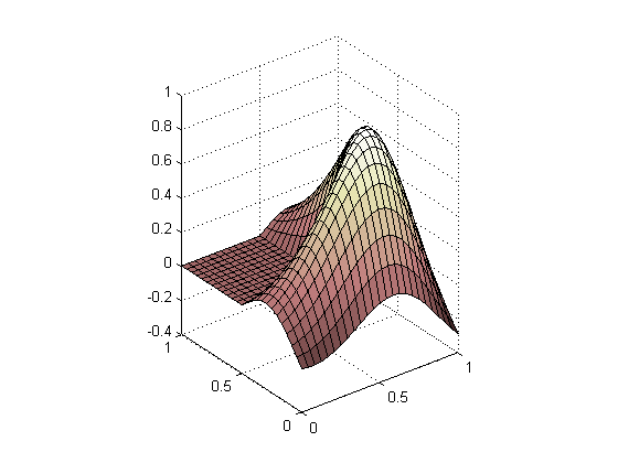
The most natural way to create surface plots in MATLAB is to use a matrix of height values. Consider the surface plot of the MathWorks logo, based on the L-shaped membrane.

n = 12; % number of partitions in each dimension.
[X,Y] = meshgrid(linspace(0,1,2*n+1));
L = (40/51/0.9)*membrane(1,n);
surf(X,Y,L);
colormap pink;
set(gca,'dataAspectRatio', [1 1 1]);

The first step in translating a matrix-based plot into an STL-file is to break up each square element in the mesh into two triangular elements. We can make use of the function DELAUNAY to create a Delaunay triangulation of the rectilinear mesh.

faces   = delaunay(X,Y);
patches = trisurf(faces,X,Y,L);
set(gca,'dataAspectRatio', [1 1 1]);

Notice that this mesh has no thickness, so it cannot yet be used to make a solid 3D print. We can make a shell out of this surface as follows. First, project all the vertices of the triangles downward along normal vectors to create a second surface with no thickness beneath the original. Then connect the two surfaces along their boundaries to define a third surface.

Let us begin by creating a 3-by-3-by-n tensor called ‘facets’ that will allow us to easily index through the 3 cartesian coordinates of the 3 vertices of the n triangles that make up our surface.

vertices = get(patches,'vertices');
facets = vertices';
facets = reshape(facets(:,faces'), 3, 3, []);

We will say that the normal at a vertex is the average of the normals to the facets that share this vertex. So, we will need to know the normals for each facet. We can calculate the normals of each facet by taking the cross-product of two edges of the facet, taking note of their orientation to ensure that the normals of the whole surface are consistent.

% SQUEEZE compacts empty dimensions.
edge1 = squeeze(facets(:,2,:) - facets(:,1,:));
edge2 = squeeze(facets(:,3,:) - facets(:,1,:));
normals = edge1([2 3 1],:) .* edge2([3 1 2],:)...
        - edge2([2 3 1],:) .* edge1([3 1 2],:);
normals = bsxfun(@times,...
  normals, 1 ./ sqrt(sum(normals .* normals, 1)));

We can compute the normal at each vertex by averaging the normals of its neighboring facets.

meanNormal = zeros(3,length(vertices)); % pre-allocate memory.
for k = 1:length(vertices)
  % Find all faces shared by a vertex
  [sharedFaces,~] = find(faces == k);
  % Compute the mean normal of all faces shared by a vertex
  meanNormal(:,k) = mean(normals(:,sharedFaces),2);
end
meanNormal = bsxfun(@times, meanNormal,...
  1 ./ sqrt(sum(meanNormal .* meanNormal, 1)));

Now we merely need to copy and shift all of the vertices downward along their normals. we will call these new vertices ‘underVertices’.

shellThickness = 0.05;
underVertices  = vertices - shellThickness*meanNormal';

Let us see what we have got so far.

underFaces = delaunay(underVertices(:,1),underVertices(:,2));
trisurf(underFaces,...
   underVertices(:,1),...
   underVertices(:,2),...
   underVertices(:,3));
set(gca,'dataAspectRatio', [1 1 1],...
  'xLim',[0 1],'yLim',[0 1]);

Notice that there are some extra facets that we did not intend. These arise from the 2D Delaunay triangulation, which connects vertices contained within the convex hull of the whole set of vertices by default. This did not pose a problem in our original surface because the boundaries consisted of a square, which is its own convex hull. The boundary of our new surface is the original square boundary deformed by the translation of each vertex through the normal vectors we calculated. Thus, our new surface has a boundary that is not its own convex hull. MATLAB’s DELAUNAYTRI class allows us to specify the boundary in 2D, which solves our problem.

To resolve this problem, we will first find the indices of the boundaries of the original surface, which will also index the boundaries of the lower surface. These boundary indices will serve to constrain the Delaunay triangulation and will be used to connect the two surfaces with a new surface. First, let us find the boundary indices.

boundaryIndices = ...
 [find(vertices(:,2) == min(vertices(:,2))); % min y
  find(vertices(:,1) == max(vertices(:,1))); % max x
  find(vertices(:,2) == max(vertices(:,2))); % max y
  find(vertices(:,1) == min(vertices(:,1)))];% min x

Next we will rearrange the indices so they parameterize the boundary. That is, we traverse the boundary in a counterclockwise sense as the index increases.

boundaryIndices = [...
  boundaryIndices(1:floor(end/4-1)); % semi open interval [1, end/4).
  boundaryIndices(floor(end/4+1):floor(end/2));%[end/4, end/2)
  boundaryIndices(floor(end*3/4-1):-1:floor(end/2+1));%[end/2,end*3/4)
  boundaryIndices(end-1:-1:floor(end*3/4+1))]; %[end*3/4, end)

The DELAUNAYTRI constructor expects each constrained edge to be defined in terms of its terminal vertices. We can create a sequence of edges by staggering the boundary vertices.

constrainedEdges = [boundaryIndices(1:end-1), boundaryIndices(2:end)];
underFaces = DelaunayTri(...
  [underVertices(:,1),underVertices(:,2)],constrainedEdges);

The DELAUNAYTRI constructor has created a triangulation that consists of two parts: one region within our constrained edges, and another outside of them. Since we only care about the inside region, we will pick it out.

inside = underFaces.inOutStatus; % 1 = in, 0 = out.
underFaces = underFaces.Triangulation(inside,:);

The normals of the lower surface have the same orientation as the original surface because of the way we constructed it. However, we will be making a closed surface by connecting these two, at which point the normals of the lower surface will need to be reversed to point outward. So, let us flip the lower surface’s normals.

underFaces = fliplr(underFaces);

Let us see what we have got so far.

trisurf(underFaces,...
   underVertices(:,1),...
   underVertices(:,2),...
   underVertices(:,3));
set(gca,'dataAspectRatio', [1 1 1],...
  'xLim',[0 1],'yLim',[0 1]);

This looks much better. Now we can move on to connect these two surfaces with a third surface that we will call ‘wall’. The wall will be made up of the boundary vertices of the top and bottom surfaces. We will triangulate these vertices by defining each facet of the wall to have one vertex on one surface and two vertices on the other surface.

wallVertices = [vertices(boundaryIndices,:);
           underVertices(boundaryIndices,:)];
% Number of wall vertices on each surface (nwv).
nwv          = length(wallVertices)/2;
% Allocate memory for wallFaces.
wallFaces    = zeros(2*(nwv-1),3);
% Define the faces.
for k = 1:nwv-1
  wallFaces(k      ,:) = [k+1  ,k      ,k+nwv];
  wallFaces(k+nwv-1,:) = [k+nwv,k+1+nwv,k+1];
end

Let us see what we have got so far.

trisurf(wallFaces,...
   wallVertices(:,1),...
   wallVertices(:,2),...
   wallVertices(:,3));
set(gca,'dataAspectRatio', [1 1 1],...
  'xLim',[0 1],'yLim',[0 1]);

Now let us assemble our three surfaces into one closed surface that we will call ‘shell’.

% Shift indices to concatenate with the original surface.
underFaces = underFaces +   length(vertices);
wallFaces  = wallFaces  + 2*length(vertices);
% Concatenate the results.
shellVertices = [vertices; underVertices; wallVertices];
shellFaces    = [faces;    underFaces;    wallFaces];

Most 3D printers require that all of the vertex coordinates be non-negative, so we will shift our shell up to satisfy this convention.

minZ = min(shellVertices(:,3));
shellVertices = shellVertices...
  - repmat([0 0 minZ],length(shellVertices),1);

Let us look at the final result.

trisurf(shellFaces,...
   shellVertices(:,1),...
   shellVertices(:,2),...
   shellVertices(:,3));
set(gca,'dataAspectRatio', [1 1 1],...
  'xLim',[0 1],'yLim',[0 1]);

The final stage is to convert this surface into an STL-file. We refer to the excellent entry in the File Exchange called stlwrite for converting our surface to an STL-file. Stlwrite is suitable for closed surfaces defined by data, but not for surfaces with boundaries like the one we started with here, because stlwrite will generate a mesh with no thickness.

% Name your STL-file
filename = 'MathWorksLogo.stl';

% Create the facets.
shellFacets = shellVertices';
shellFacets = reshape(shellFacets(:,shellFaces'), 3, 3, []);

% Compute their normals.
edge1 = squeeze(shellFacets(:,2,:) - shellFacets(:,1,:));
edge2 = squeeze(shellFacets(:,3,:) - shellFacets(:,1,:));
shellNormals = edge1([2 3 1],:) .* edge2([3 1 2],:)...
        - edge2([2 3 1],:) .* edge1([3 1 2],:);
shellNormals = bsxfun(@times,...
  shellNormals, 1 ./ sqrt(sum(shellNormals .* shellNormals, 1)));

% Associate each facet with its normal.
shellFacets = cat(2, reshape(shellNormals, 3, 1, []), shellFacets);

% Open the file for writing
fid = fopen(filename,'wb+');

% Write the file contents.
% Write HEADER.
fprintf(fid,'solid %s\r\n',filename);
% Write DATA.
fprintf(fid,[...
'facet normal %.7E %.7E %.7E\r\n' ...
'outer loop\r\n' ...
'vertex %.7E %.7E %.7E\r\n' ...
'vertex %.7E %.7E %.7E\r\n' ...
'vertex %.7E %.7E %.7E\r\n' ...
'endloop\r\n' ...
'endfacet\r\n'], shellFacets);
% Write FOOTER.
fprintf(fid,'endsolid %s\r\n',filename);

% Close the file.
fclose(fid);

MATLAB Materialized

With your STL-file in hand, you can now make your print! If you do not have your own 3D printer, you can look for your nearest maker-space to see if they have one, or send your STL-file off to a 3D printing service provider such as Shapeways, Ponoko, Sculpteo, I.Materialize, ZoomRP, or RedEye. I am a member of the maker-space Artisan’s Asylum, which has a nice 3D printer, among many other tools. Here is a photo of my completed L-shaped membrane.

Good luck and have fun turning your MATLAB plots into tangible objects!

Published with MATLAB® R2013a