Evaluating deep learning model performance can be done a variety of ways. A confusion matrix answers some questions about the model performance, but not all. How do we know that the model is identifying the right features?
Let's walk through some of the easy ways to explore deep learning models using visualization, with links to documentation examples for more information.
Background: Data and Model Information
For these visualizations, I'm using models created by my colleague Heather Gorr. You can find the code she used to train the models on GitHub here.
The basic premise of the models and code is using wildlife data to see if MATLAB can be used to correctly identify classes of animals in the wild. The sample images look something like this:
Bear
 |
Bear
 |
Bear
 |
Bighorn Sheep
 |
Bighorn Sheep
 |
Cow
 |
Cow
 |
Coyote
 |
Coyote
 |
Dog
 |
The two models I will use today were trained on the following classes of images:
- [ Bear | Not-Bear ] All bears should be classified as "bear", anything else should be "not bear"
- [ Bear | Cow | Sheep ]: 3 classes of animals that must fit into the categories
Here are the sample images run through each network.
Bear | Not-Bear Classifier (net1)
| bear
|
bear
|
bear
|
not bear
|
not bear
|
| not bear
|
not bear
|
not bear
|
not bear
|
not bear
|
Bear | Cow | Sheep Classifier (net2)
| bear
|
bear
|
bear
|
bighorn sheep
|
bighorn sheep
|
| cow
|
cow
|
bear
|
bear
|
cow
|
You now can see that most predictions are correct, but once I add in a few animals not in the expected categories, the predictions get a little off. The rest of this post is using visualization to find why the models predicted a certain way.
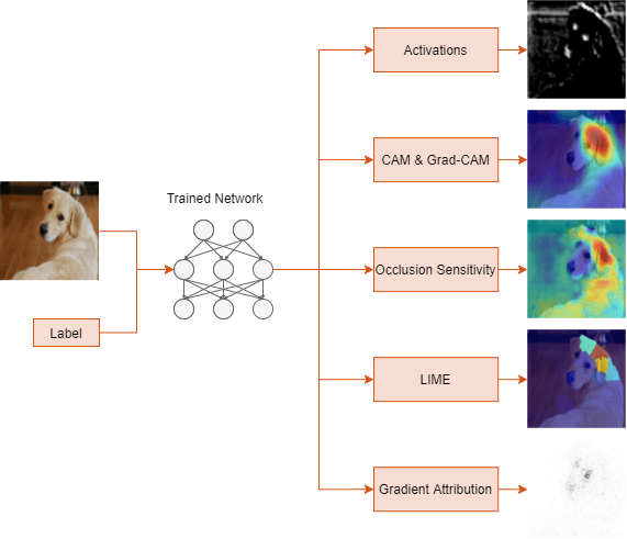
Popular Visualization Techniques
...and how to use them
Techniques like LIME, Grad-CAM and Occlusion Sensitivity can give you insight into the network, and why the network chose a particular option.
LIME
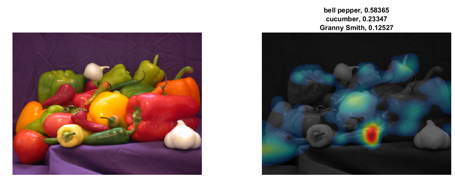
imageLIME is newer technique added to MATLAB in 2020b. Let's investigate the coyote that was called a bear:
Start by displaying the predictions and the confidences.
[YPred,scores] = classify(net2,img);
[~,topIdx] = maxk(scores, 3);
topScores = scores(topIdx);
topClasses = classes(topIdx);

figure; imshow(img)
titleString = compose("%s (%.2f)",topClasses,topScores'); %'
title(sprintf(join(titleString, "; ")));
|
 |
Then, use imageLime to visualize the output.
map = imageLIME(net2,img,YPred);

figure
imshow(img,'InitialMagnification',150)
hold on
imagesc(map,'AlphaData',0.5)
colormap jet
colorbar

title(sprintf("Image LIME (%s)", YPred))
hold off
|
 |
|
Here, imageLIME is indicating the reason for the prediction is in the lower corner of the image. While this is clearly an incorrect prediction, the strongest features are not surrounding the coyote. This would indicate those features were learned incorrectly for the bear class. |
Grad-CAM
Let's focus on the bears using Grad-CAM, another visualization technique available. Here I think you'll find some very interesting things about the models we're using.
Keep in mind - net1 detects bear or not-bear, and net2 detects bear, cow or sheep.
Let's set up for Grad-CAM.
lgraph = layerGraph(net2);
lgraph = removeLayers(lgraph, lgraph.Layers(end).Name);
dlnet = dlnetwork(lgraph);
softmaxName = 'predictions_softmax';
featureLayerName = 'activation_94_relu';
[classfn,score] = classify(net1,img);
imshow(img);
title(sprintf("%s (%.2f)", classfn, score(classfn)));
dlImg = dlarray(single(img),'SSC');
[featureMap, dScoresdMap] = dlfeval(@gradcam, dlnet, dlImg, softmaxName, featureLayerName, classfn);
gradcamMap = sum(featureMap .* sum(dScoresdMap, [1 2]), 3);
gradcamMap = extractdata(gradcamMap);
gradcamMap = rescale(gradcamMap);
gradcamMap = imresize(gradcamMap, inputSize, 'Method', 'bicubic');
Running this code for bears 1,2 and 3, using the bear, not-bear model, here are the results:
Nothing too exciting with the images above. Those are definitely bears, and the visualization is more or less targeting the bear.
NOW! Let's use the other model. [Same code as above, just replacing net1 with net2] Remember at the very beginning: The network predicted all bears correctly as bears. So why spend time to visualize correct results?
Do you see it? This model is always activating on the lower left corner! So the model is predicting correctly, but why it predicted a bear is suspect.
One more thing before we move on: what if we just crop out the strongest/incorrect features the network is focused on?
 ... interesting! Removing the strongest features in the image caused the network to predict incorrectly. This means the network is not likely learning real animal features, and focused on other aspects of the images. Most often I find that visualizations are great to gain insight into a model, but rarely have I been able prove an "accurate" model is not really predicting accurately at all!! My work here is done.
Occlusion Sensitivity
The final output visualization we'll cover today is occlusion sensitivity. This is by far the easiest to implement code-wise.
label = classify(net1,img);

scoreMap = occlusionSensitivity(net1,img,label);

figure
imshow(img)
hold on
imagesc(scoreMap,'AlphaData',0.5);
colormap jet
 Here you can see that the reason the sheep is labeled "not bear" is in the center of the animal. I was semi-disappointed to not have those big horns light up, but what can you do?
Gradient Attribution Techniques
Just another note that there are more visualization techniques, such as Gradient Attribution Techniques, but I think we covered a lot already. To learn more, you can check this doc example.
Inside the Network Insights
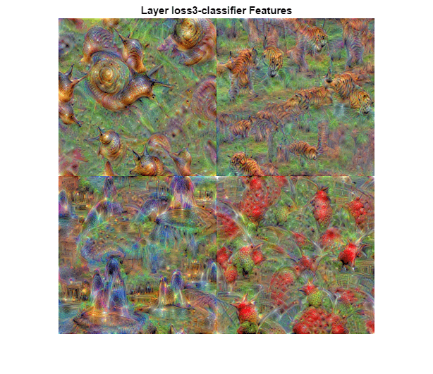
Deep Dream
Here we can visualize the network's learned features. Let's visualize the first 25 features learned by the network at the second convolutional layer.
layer = 'conv2d_2';
channels = 1:25;

I = deepDreamImage(net2,layer,channels, ...
    'PyramidLevels',1, ...
    'Verbose',0);

figure
for i = 1:25
    subplot(5,5,i)
    imshow(I(:,:,:,i))
end
|
 |
I'll be honest, while I find deep dream visually pleasing, I don't tend to use this very often as a debugging technique, though I'd be interested to hear from anyone who has an example of success. Sometimes, deep dream can be helpful for later layers of the network, where other techniques will certainly fail.
However, in this particular example, I wasn't able to find anything particularly appealing even after running deep dream for 100 iterations.
iterations = 100;
layerName = 'new_fc';

I = deepDreamImage(net1,layerName,1, ...
    'Verbose',false, ...
    'NumIterations',iterations);

figure
imshow(I)

This image is visualizing the "bear" class. I'm not seeing particularly insightful to comment on, though I have seen very attractive deep dream images created from other pretrained networks in this example.
Activations
Similar to deep dream, you can use activations to visualize the input image after it passes through specific channels, which are showing the learned features from the network.
im = imread('bear2.JPG');

imgSize = size(im);
imgSize = imgSize(1:2);

act1 = activations(net1,im,'conv2d_7');

sz = size(act1);
act1 = reshape(act1,[sz(1) sz(2) 1 sz(3)]);

I = imtile(mat2gray(act1),'GridSize',[7 7]);
imshow(I)
 Then, you can use activations to quickly pull the strongest channel activating.
[maxValue,maxValueIndex] = max(max(max(act1)));
act1chMax = act1(:,:,:,maxValueIndex);
act1chMax = mat2gray(act1chMax);
act1chMax = imresize(act1chMax,imgSize);
I = imtile({im,act1chMax});
imshow(I)
 See a related documentation example for more ways to use activations.
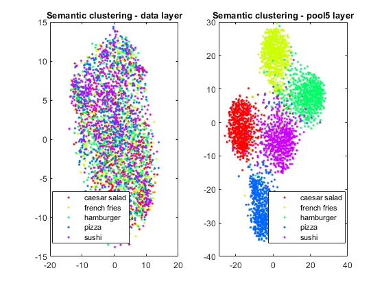
TSNE
Maria wrote a blog post about this a while back, and I'm happy to report a new example is in documentation here. This can help show similarities and differences between classes.
 Any other visualizations you like that I should add to this collection? Let me know in the comments below!


Comments
To leave a comment, please click here to sign in to your MathWorks Account or create a new one.