
MATLAB’s Best Model: Deep Learning Basics
This post is from Heather Gorr, MATLAB product marketing. You can follow her on social media: @heather.codes, @heather.codes, @HeatherGorr, and @heather-gorr-phd. This blog post follows the fabulous modeling competition LIVE on YouTube, MATLAB's Best Model: Deep Learning Basics to guide you in how to choose the best model. For deep learning models, there are different ways to assess what is the “best” model. It could be a) comparing different networks (problem 1) or b) finding the right parameters for a particular network (problem 2).
How can this be managed efficiently and quickly? Using a low code tool in MATLAB, the Experiment Manager app!
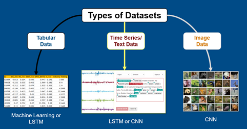 Fig 1: Common data sets and networks
We used doc examples for repeatability (plus, reasonably sized data sets for a livestream!) and used apps in MATLAB to explore, train, and compare the models quickly. We'll discuss more as we get into the details!
Fig 1: Common data sets and networks
We used doc examples for repeatability (plus, reasonably sized data sets for a livestream!) and used apps in MATLAB to explore, train, and compare the models quickly. We'll discuss more as we get into the details!
Fig 2: Convolutional Neural Network (CNN) diagram
As you may recall from previous posts, we have some great starting points in this field! We used transfer learning, where you update a pretrained network with your data.
Fig 3: Pretrained models in Deep Network Designer
We wanted varying levels of complexity for our competition, so we decided on squeezenet, googlenet, and inceptionv3.
Fig 4: Setting network parameters in Experiment Manager App
As you probably know, training networks can take some time! Here we are training 3 of them - so you want to consider your hardware and problem before hitting run. You can adjust setting to use GPUs and run experiments in parallel easily through the app.
I started the experiment a bit early to ensure we had time to compare and ran it on my Linux machine for multi-GPU action!
Fig 5: Classification results in Experiment Manager App
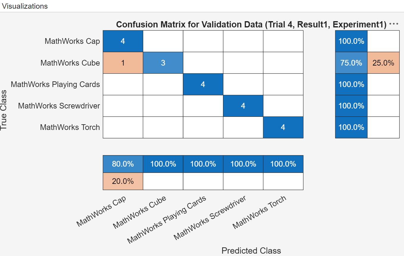
We found that in this example, inceptionv3 performed best in terms of accuracy (91.9 %) but takes much longer as it’s a more complicated architecture compared to the others. Looking at the next runners-up, googlenet might be a better compromise since it was much faster and still has similarly good validation accuracy (91%). The squeezenet model trained the fastest but has worse accuracy, though I wouldn't rule it out! Every problem is different when it comes to what’s most important! Finally, we checked the confusion matrices which looked quite similar and balanced. This is a very important visual to help ensure you don’t have imbalanced accuracies amongst classes... which leads us to our last criteria.
Fig 6: Exploring results in Experiment Manager App
We ran the experiment and googlenet performed much better here (though obviously took longer to train). It's interesting that there is no clear difference in accuracy when comparing the solvers - more data would likely help examine this. However, the solvers made a big difference in the default algorithm with minimal layers (70 vs 80%). This is the type of situation worth checking into if you see such variation!
Fig 7: Comparison of RNN (left) and LSTM network (right)
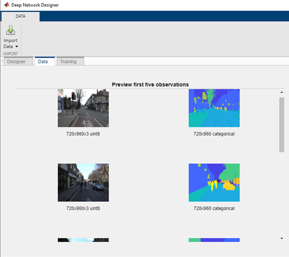
With LSTMs, you often don’t need as many layers as CNNs - the art is in choosing parameters to best represent the data and trends. While I’ve encountered very deep LSTMs, most often the network can learn well with very few layers. For example, the Deep Network Designer has a template with 6 layers: input, lstm, dropout, fullyConnected, softmax, and a classification or regression layer. This is a straightforward architecture where the data prep and layer parameters have a lot of influence.
Fig 8: Deep Network Designer 6 layer template
We use the same approach as above to compare different network parameters using the Experiment Manager and a doc example predicting remaining useful life (RUL) of an engine:
Fig 9: Comparing main network parameters
A custom metric was used MeanMaxAbsoluteError, which is helpful as you could include any methods you like to judge the goodness-of-fit. We checked the setupfunction, ran the experiment, and anxiously awaited the results!
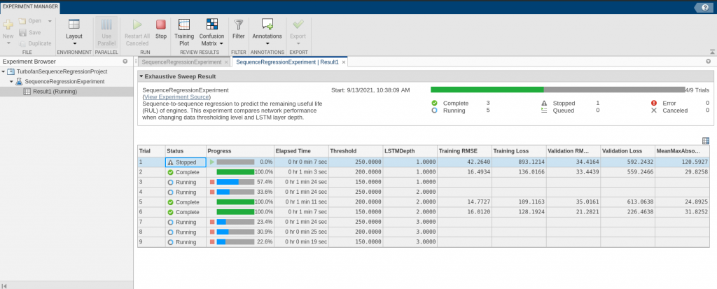 Fig 10: Running the experiment and comparing results
Fig 11: RMSE results
The best model (with minimal RMSE) is the network with the smallest threshold (150) and smallest depth (1). In this case, there wasn't any improvement in the results based on depth of the network, so again simplicity is something to consider when setting up your LSTMs and will help with explainability as noted above.
There are excellent examples in the doc to show LSTM training and assessment in more details for several problems including video, audio, and text. Sadly, we couldn’t do more comparisons in an hour but maybe next time we can get into more complicated problems now that we've covered the basics! Check out more examples here.

Approach
We created two problems for image classification and timeseries regression. Based on the data sets, we considered two types of models: Convolutional (CNN) and Long Short-Term Memory (LSTM) networks. The image below shows some common networks used for different data types.
Fig 1: Common data sets and networks
We used doc examples for repeatability (plus, reasonably sized data sets for a livestream!) and used apps in MATLAB to explore, train, and compare the models quickly. We'll discuss more as we get into the details!
Problem 1: Image classification
For our first problem, we compared CNN models to classify types of flowers. CNNs are very common as they involve a series of operations, which we can generally understand: convolutions, mathematical operations, and aggregations.
Choosing networks
We started by exploring pretrained models using the Deep Network Designer app which provides a sense of the overall network architecture to help us select before investigating the detail.
Comparing networks
Next, we needed to train and validate all 3 networks and compare the results! The Experiment Manager app is super helpful to stay organized and automate this part. This doc example walks through setting up and running the experiment:cd(setupExample('nnet/ExpMgrTransferLearningExample'));setupExpMgr('FlowerTransferLearningProject');

The judges' scores
How did our models perform? There are a few criteria we used to assess:- Accuracy
- Speed
- Overall quality
- Explainability

Explainability
Being able to interpret the models is increasingly important, and model explainability is an area of active research in the field of deep learning. We'll keep this section brief as we have a lot more to come on these topics. Basically, you understand what's happening, especially if something goes wrong (the developer, the team, even the users need to understand). There are some good techniques such as Network Activations and Visualizations, and other strategies. A few last tips - be sure to document well, and if you've used a pretrained model, make sure the training data and model info are transparent and unbiased.Tuning
A huge part of deep learning is tuning the networks once you are satisfied with the approach. There are many parameters to adjust for improvements in the layer architecture, solvers, and data representation. Again, the apps will help with this as you can examine and adjust the parameters easily in Deep Network Designer, then perform a parameter sweep using the Experiment Manager. We followed a doc example which shows trying three solvers with googlenet and a simple 'default' network:cd(setupExample('nnet/ExperimentManagerClassificationExample'));setupExpMgr('MerchandiseClassificationProject');
We won’t get into the details of available solvers in this post, but this is a great way to explore if you forget the difference between Stochastic Gradient Descent with Momentum (sgdm) and Root Mean Square Propagation (RMSProp) off hand! There's a lot more in the doc including a quick overview all parameters available to tune.

Problem 2: Time series regression
Next we focused on the timeseries regression problem. First, let’s think about the overall architecture. CNNs are broadly useful for many problems, but there are times when the model needs to know info from previous time steps. This is where Recursive Neural Networks (RNN) come in handy as they retain memory through the system which makes them well-suited to timeseries, video, text, and other sequential problems. In deep learning terminology, CNNs are feed forward, while RNN's are feed backward to carry some memory through the inputs and outputs of the layers. In this case, we looked specifically at LSTM which is an RNN with extra gates for inputs and outputs. This facilitates retaining longer-term trends in the data, important for time series problems. The illustration below compares the two networks.

cd(setupExample('nnet/ExperimentManagerSequenceRegressionExample'));setupExpMgr('TurbofanSequenceRegressionProject');
Selecting parameters
We compared two main network parameters: the threshold and LSTM depth. The threshold represents a cutoff value for the response data and the LSTMDepth is the number of layers. Fig 10: Running the experiment and comparing results
The judges' scores
With regression problems, where a numeric value is predicted, the common measure of accuracy is RMSE (root mean squared error) between known and predicted data. Ideally, the RMSE is as close to zero as possible.
Summary
We were able to train, compare and assess these beautiful models (in under an hour!) Hopefully this can give you a sense of how to choose networks for your data and how to set up experiments to tune and compare the networks. Using the apps and carefully thinking about the criteria are super helpful during this process. If you’d like to learn more about setting up your own experiments, visit these 2 video tutorials from Joe Hicklin. We'll be back again for our modeling competition series - subscribe to the @matlab YouTube channel to stay tuned for more and stay connected on social media and in the comments. Let us know what you'd like to see next!- Category:
- Deep Learning


Comments
To leave a comment, please click here to sign in to your MathWorks Account or create a new one.