Gourds to Graphics: The MATLAB Pumpkin

Posted by Adam Danz, October 31, 2023

12 views (last 30 days) | 0 Likes | 0 comment

Today's graphics adventure is written by Eric Ludlam, development manager of MATLAB's Charting team. Eric has a whopping 27 years of experience working in MATLAB Graphics, starting in MATLAB 5.0! Eric is renowned within MathWorks for his love of trebuchets, catapults and Punkin Chunkin. His exceptional graphics demos have appeared in MathWorks' Community blog, MATLAB blog, and in MATLAB social media feeds. Today he answers the collective question we all have. How'd you do that?

The MATLAB social media team has been sharing images and code for different pumpkins around Halloween time for the past couple years, and these gourds have been pretty popular. One question asked in the comments was how the pumpkin was designed. Today I'd like to explain the types of decisions made while developing the code and share some fun tricks with vectorization and implicit expansion for anyone just learning how to write efficient code in MATLAB.

The pumpkin I'd like to use today is a speckled yellow and orange pumpkin I picked up locally here in Massachusetts. Here's a picture of our target pumpkin:

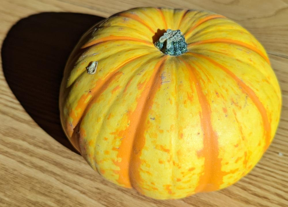
There are a few interesting features of this pumpkin, including a stubby little stem, 2 sets of creases/bumps, a 2-tone color scheme where the 2nd color is in the deeper crease, and speckles. A bunch of fun challenges!

Before we start let's review the various components of our algorithm. We can break the overall shape of our pumpkin into 2 major parts, the semi-spherical pumpkin part, and the stem.

The algorithm for the pumpkin part is made of 3 key components which will be combined together into one set of matrices drawn with the surf command.

Unit Sphere of the underlying shape
Creases and bumps as seen around the circumference
Dimple on the top and bottom

I'll start describing how to make the patterns for creases, bumps, and the dimple for the pumpkin, then move to how the stem is made before combining it all at the end.

Computing Creases and Bumps

In this article, I'll use "crease" to describe an indentation that travels from the stem to the bottom of the pumpkin. I'll use the term "bump" to generally refer to one pattern that runs from crease-to-crease around the circumference.

There is one set of creases that are deeper (and more orange) than the other. I'll call a deep crease the 'primary' crease, and the other is the 'secondary' crease. Since these creases are mapped onto a sphere, there are the same number of bumps as there are creases. To develop a crease/bump pattern we need a way to create a repeating pattern numerically. To do this we need to set up a few parameters, including how many bumps there are, and how many vertices we'd like in our graphic.

I count around 10 creases, with secondary crease between each one. We also want to select enough vertices per bump to provide a smooth look across the pumpkin. I tried a few different values for vertices per bump and found that 10 looks good while still being a small number when multiplied out against the total number of bumps. We don't want too many vertices because this number also impacts the size of the speckles which we'll see at the end, and our target pumpkin has big spots.

We can compute our total number of vertices from the total number of bumps, and use that size for the combined set. The +1 for numVerts is because the first and last vertex around the sphere are shared, which will align the creases with a vertex so they look sharp.

numPrimaryBumps = 10;

totalBumps = numPrimaryBumps*2; % Add in-between creases.

vertsPerBump = 10;

numVerts = totalBumps*vertsPerBump+1;

Next, we need to compute the depth of the creases for both the primary and secondary creases. We'll specify the depth in terms of a unit sphere. To create our pattern vector we'll start with a linear list of values and use mod(x, 2) to create the repeating pattern which means we start with values from 0 to the number of bumps*2.

rPrimary = linspace(0,numPrimaryBumps*2,numVerts);

rSecondary = linspace(0,totalBumps*2,numVerts);

Next, we'll define some depths for the creases. The depth of the primary crease will be the sum of crease_depth and crease_depth2, so we need to keep that in mind while selecting depth values.

The bump vectors Rxy_primary and Rxy_secondary represent the change in radius of our unit sphere in the xy plane. mod is used to create a repeating pattern between [ 0 2 ]. That pattern needs to be shifted to [ -1 1 ] so that when the result is squared, it creates a curve.

crease_depth = .04;

crease_depth2 = .01;

Rxy_primary = 0 - (1-mod(rPrimary,2)).^2*crease_depth;

Rxy_secondary = 0 - (1-mod(rSecondary,2)).^2*crease_depth2;

Rxy = Rxy_primary + Rxy_secondary;

Let's plot the result in polar coordinates so we can get a feel for what it will look like. When plotting, add 1 to the radius to simulate how we'll be adding the pumpkin's core diameter to this crease pattern.

polarplot(Rxy+1, 'LineWidth',2);

rlim([0 1.1])

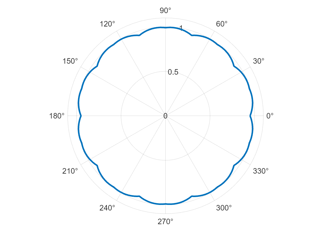
The secondary bump looks shallow in this diagram, but that is roughly what I found on the real pumpkin.

Speaking of which, let's take a quick look at what we have so far by multiplying Rxy to the X & Y coordinates of a sphere.

[ Xsphere, Ysphere, Zsphere ] = sphere(numVerts-1); % Sphere creates +1 verts

Xpunkin = (1+Rxy).*Xsphere;

Ypunkin = (1+Rxy).*Ysphere;

surf(Xpunkin,Ypunkin,Zsphere)

shading interp

daspect([1 1 1])

camlight

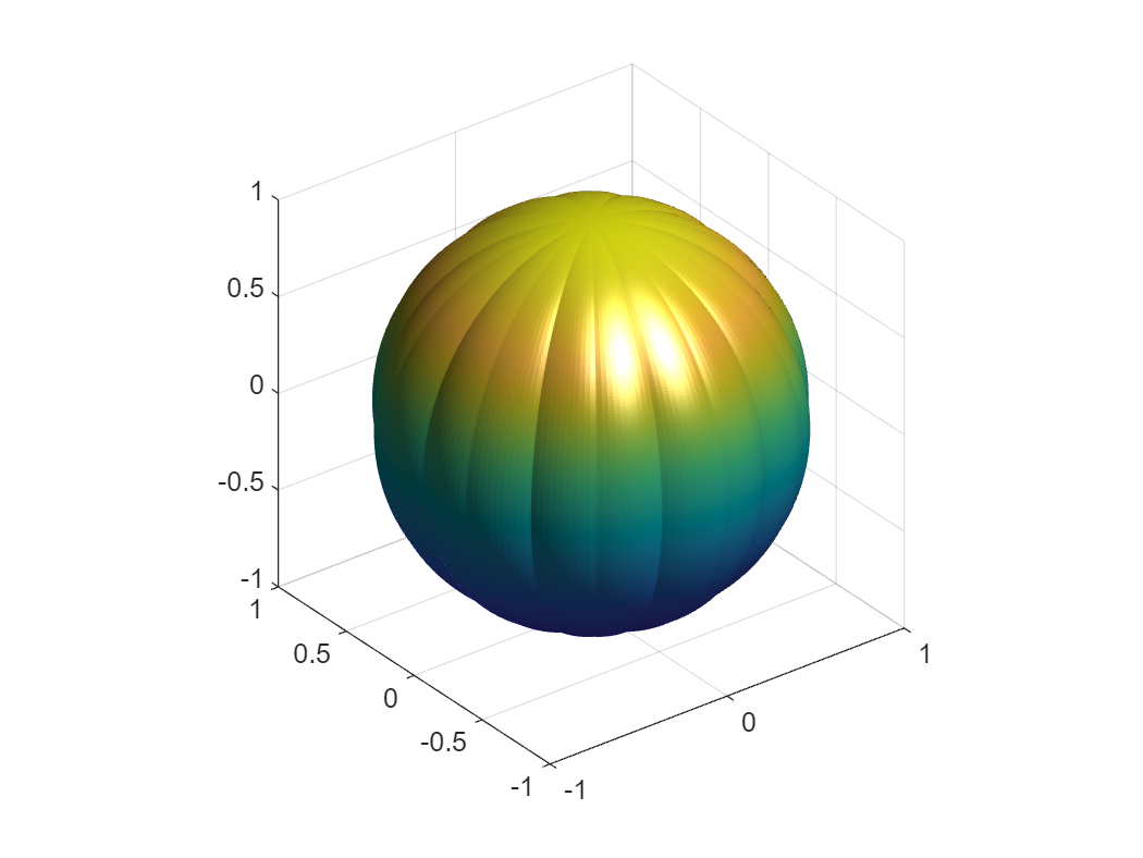
Well, this looks more like a ridgy sports ball than a pumpkin. That's because our target pumpkin has a dimple in the top and bottom.

Computing a pumpkin dimple

The dimple on a pumpkin is caused by how the fruit expands off the end of the stem as it grows. We'll use an exponential function to create the dimple as we did for the creases, but across only a single span between -1 and 1. Note also that I'm creating a column vector. That will let us apply the shape to the columns of our sphere matrix to define its vertical profile instead of applying it to the rows which would affect the bump pattern.

To see how it looks we'll plot this in polar coordinates as well, but this time I'm only showing half the polar chart since I'm computing a single profile.

dimple = .2; % Fraction to dimple into top/bottom

rho = linspace(-1,1,numVerts)';

Rz_dimple = (0-rho.^4)*dimple;

polarplot(linspace(0,pi,numVerts),Rz_dimple+1, 'LineWidth',2);

rlim([0 1.1])

thetalim([0 180])

set(gca,'ThetaZeroLocation','bottom')

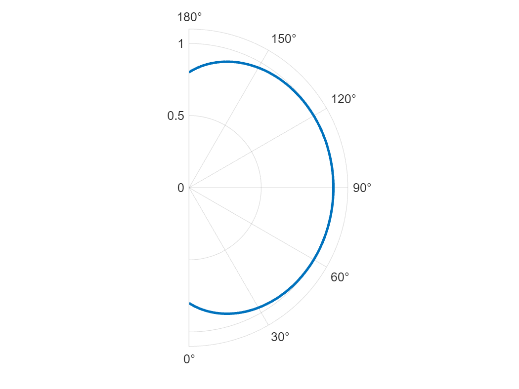
This looks a bit exaggerated in polar coordinates since the polar chart is perfectly round. When we apply it to the sphere we'll also squish it to simulate that our pumpkin is shorter than it is wide. That will give it a more natural look. I took a bit of a guess that the height of the pumpkin is just 80% of the diameter at the equator.

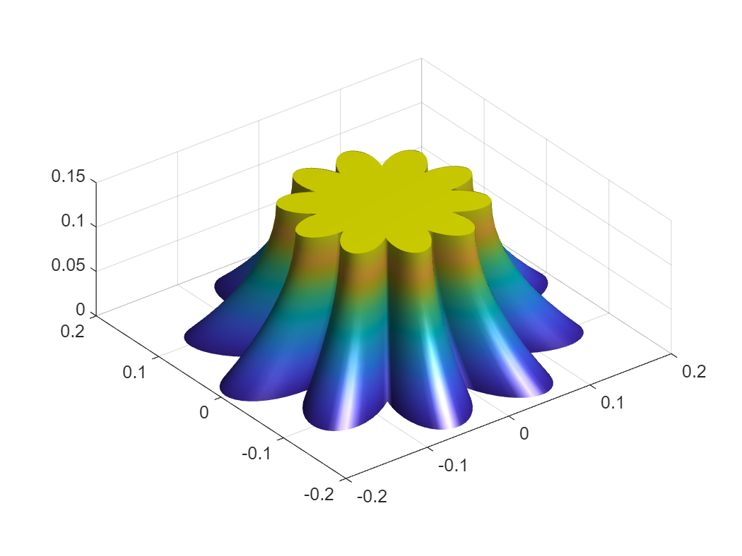
Computing the Zpunkin matrix requires adding bumps across the rows the same way as Xpunkin and Ypunkin do. It also needs the height to be adjusted, and the dimple applied on the columns. This is done using element-wise multiply .* using the row vector Rxy, and the column vector Rz_dimple.

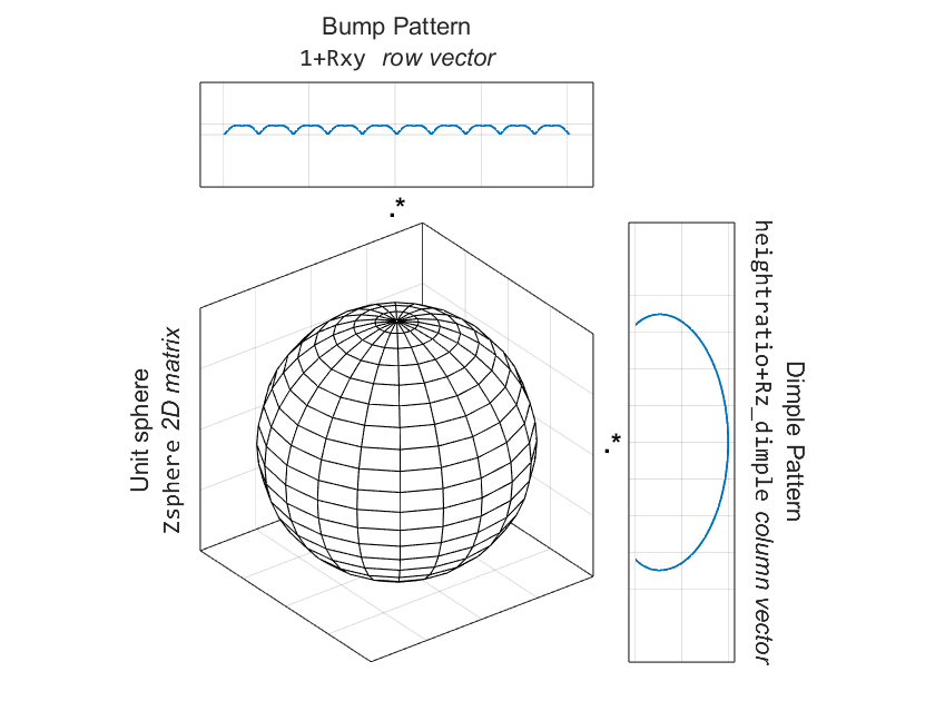
heightratio = .8;

Zpunkin = (1+Rxy).*Zsphere.*(heightratio+Rz_dimple);

%          ^bumps  ^sphere mesh ^squish 80%  ^column vector to apply dimple

surf(Xpunkin,Ypunkin,Zpunkin)

shading interp

daspect([1 1 1])

camlight

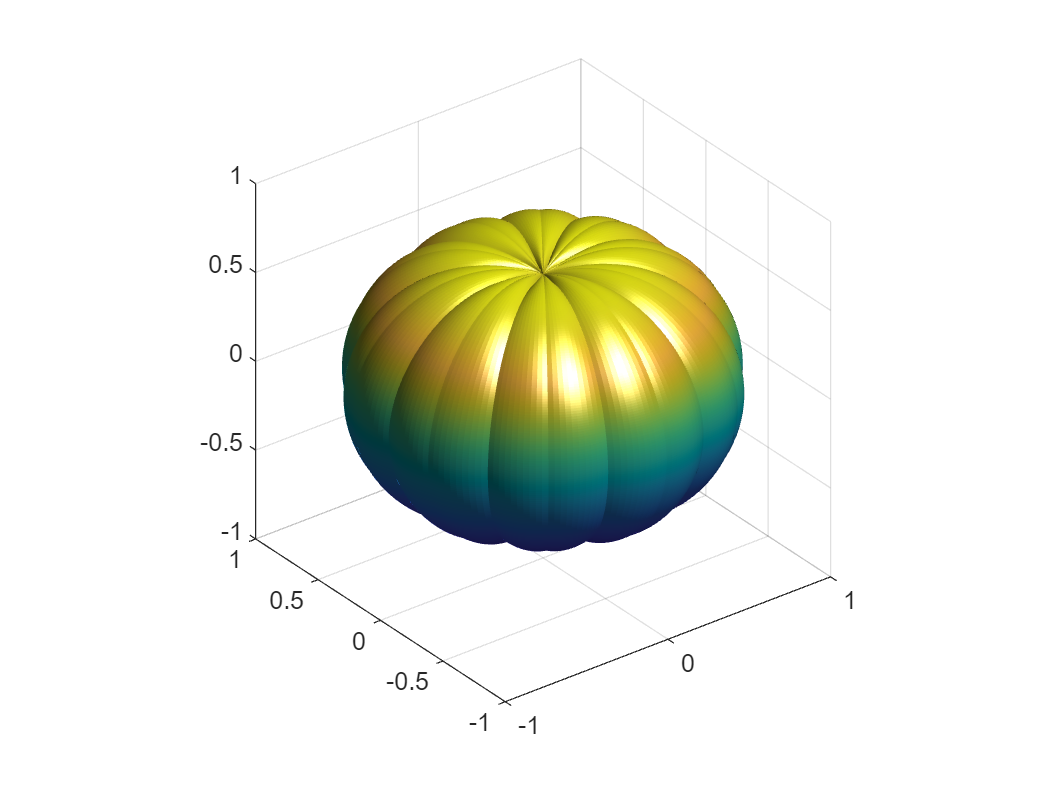
We're getting closer, but the dimple still looks a bit weird. Fortunately, we can stick a stem on there to hide that artifact.

Designing a Stem

Before starting on the stem, let's take a close look at our target pumpkin's stem:

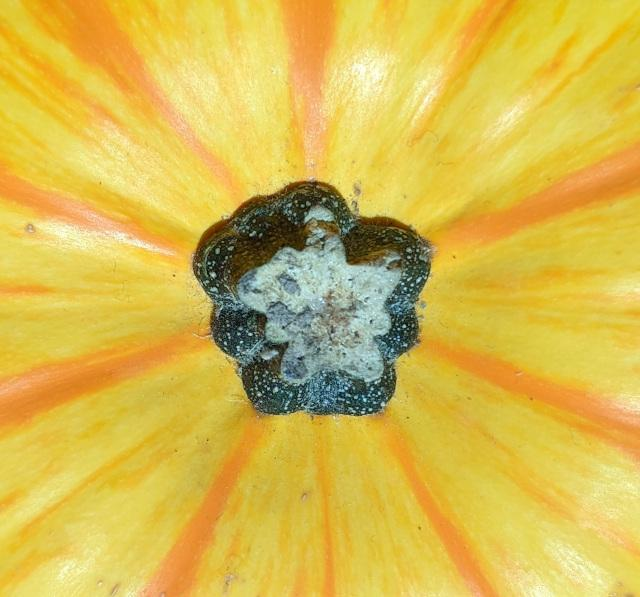
You'll notice that every bump on the stem lines up with one of the primary creases in our pumpkin! Turns out this is because the bumps that naturally occur on the stem impact the pumpkin as it grows, constraining it into a crease. For this particular pumpkin it isn't as well defined as with other breeds, and one stem bump seems to be missing top-left, but that's ok. This is MATLAB, so we'll create a perfect pumpkin stem instead.

To start, we'll create another pattern, similar to the pumpkin creases by re-using rPrimary, but offset from the pumpkin bumps by 1/2 a pattern. That way the outward bumps of the stem line up with the creases in the pumpkin.

Next, we'll create some cylinder height coordinates as Zcyl and square it to compute a curved profile so the stem is wider on the bottom than on the top.

Rstem = (1-(1-mod(rPrimary+1,2)).^2)*.05;

thetac = linspace(0,2,numVerts);

Xcyl = cospi(thetac);

Ycyl = sinpi(thetac);

Zcyl = linspace(0,1,11)'; % column vector

Rstemz = .7+(1-Zcyl).^2*.6;

Once we have these base coordinates, compute the cylindrical mesh the same way we did for the pumpkin sphere, but instead apply it to the cylinder coordinates. The row vectors Xcyl and Ycyl, when multiplied by the column vector Rstemz using element-wise multiplication operator ".*", will implicitly expand into a 2D matrix, perfect for drawing a mesh.

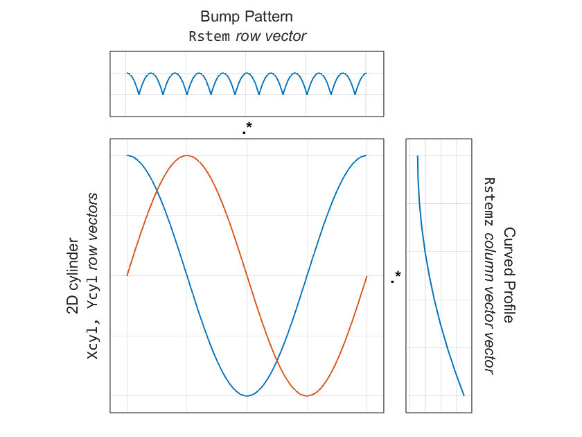
Xstem = (.1+Rstem).*Xcyl.*Rstemz;

Ystem = (.1+Rstem).*Ycyl.*Rstemz;

Zstem = repmat(Zcyl*.15,1,numVerts);

Let's take a look at our stem using a surf plot and fill in the top with a patch.

surf(Xstem,Ystem,Zstem);

shading interp

patch('Vertices', [Xstem(end,:)' Ystem(end,:)' Zstem(end,:)'],...

      'Faces', 1:numVerts, ...

      'FaceColor','y','EdgeColor','none')

lighting gouraud

daspect([1 1 1]);

camlight

This stem has a lot more definition than our target pumpkin. We'll say it's a more perfect stem.

Putting it all together!

Ok, let's put it all together! In this next code snippet, we'll re-create the pumpkin and give it a new colormap with colors selected off the photo of our target pumpkin. Then we'll add the stem but offset it by the height of our pumpkin. We'll also color the stem and stem cap based on colors also selected from the photo.

One trick in this code snippet is the creation of a colormap with only 2 colors. The validatecolor function is a new feature from R2020b that will convert valid color strings like web hex codes into RGB colors. This makes it easy to use a common color specifier in MATLAB.

Spunkin = surf(Xpunkin,Ypunkin,Zpunkin,'FaceColor','interp','EdgeColor','none');

colormap(validatecolor({'#da8e26' '#dfc727'},'multiple'));

Sstem = surface(Xstem,Ystem,Zstem+heightratio^2,'FaceColor','#3d6766','EdgeColor','none');

Pstem = patch('Vertices', [Xstem(end,:)' Ystem(end,:)' Zstem(end,:)'+heightratio^2],...

            'Faces', 1:numVerts, ...

            'FaceColor','#b1cab5','EdgeColor','none');

daspect([1 1 1])

camlight

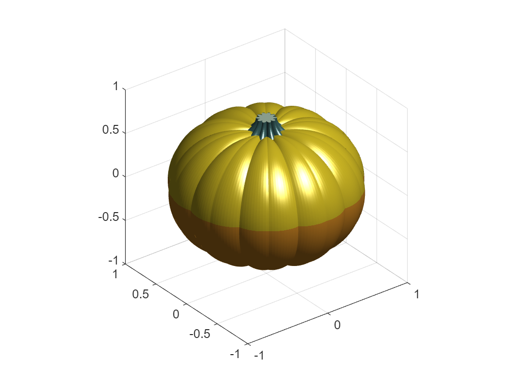
Hmm. We didn't spend any time computing where the colors would go, so by default, color is the same as Z.

Our goal is for the depths of the creases to be orange, and the bumps to be yellow, so we'll use hypot to compute distance from center as if we had a pumpkin with no dimples on the top and bottom. Let's see how that looks:

Cpunkin = hypot(hypot(Xpunkin,Ypunkin),(1+Rxy).*Zsphere); % As if pumpkin were round with no dimples

set(Spunkin,'CData',Cpunkin); % Pumpkin CData

set(Sstem,'CData',[]); % Make sure the stem doesn't contribute to auto Color Limits

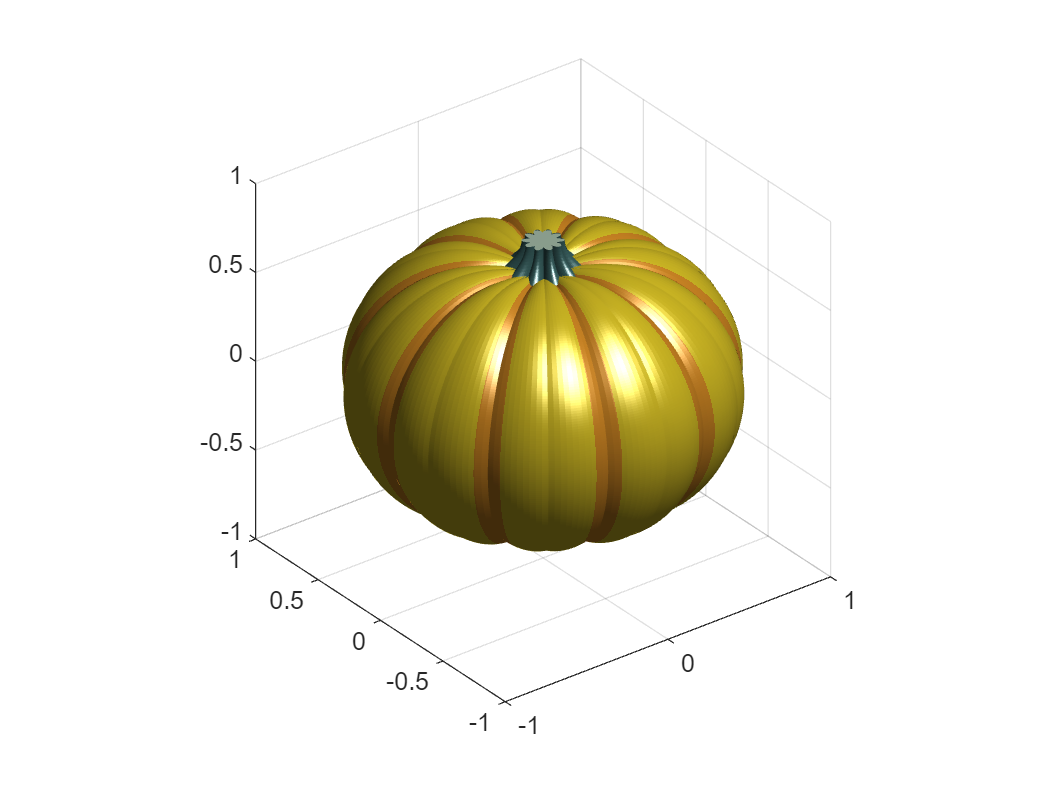
This looks too crisp due to the sharp boundary between the orange and yellow colors caused by having only 2 colors in the colormap. Fortunately, we still need to add all the speckles which we can do by adding some normally distributed random noise. Selecting the right scale for the noise took a bit of fiddling so it didn't overwhelm the bumps.

set(Spunkin,'CData',Cpunkin+randn(numVerts)*0.015);

Pumpkin Polish

The speckles mitigated the hard color boundary, so with that out of the way, we are almost done. Let's decorate by improving the lighting and material properties to give it more of a waxy light reflectance and add in more ambient light. We'll also turn off the axes and zoom in a bit.

daspect([1 1 1])

axis off

camzoom(1.8)

lighting gouraud

material([Spunkin Sstem Pstem],[ .6 .9 .3 2 .6 ])

Armed now with this vital pumpkin knowledge, what sort of gourd can you recreate in MATLAB?

Share your MATLAB Pumpkin images with us in the comments below!

Category:: Demos,; Graphics

Comments

To leave a comment, please click here to sign in to your MathWorks Account or create a new one.

MATLAB Graphics and App Building
MATLAB graphics, data visualization, and app building

MATLAB graphics, data visualization, and app building

Gourds to Graphics: The MATLAB Pumpkin

Computing Creases and Bumps

Computing a pumpkin dimple

Designing a Stem

Putting it all together!

Pumpkin Polish

Comments

Computing Creases and Bumps

Computing a pumpkin dimple

Designing a Stem

Putting it all together!

Pumpkin Polish

See Also

Comments

Select a Web Site

Americas

Europe

Asia Pacific