New Regression Capabilities in Release 2012A
This week Richard Willey from technical marketing will be guest blogging about new regression capabilities shipping with the 12a Statistics Toolbox release.
Contents
- Create a dataset
- Use linear regression to model Y as a function of X
- Use myFit for analysis
- Look for patterns in the residuals
- Look for autocorrelation in the residuals
- Look for outliers
- Use the resulting model for prediction
- Discover the full set of methods available with regression objects
- Discover the full set of information included in the regression object
- Formulas
- Modeling a high order polynomial (Option 1)
- Modeling a high order polynomial (Option 2)
- Nonlinear regression: Generate our data
- Nonlinear regression: Generate a fit
- Nonlinear regression: Work with the resulting model
- Nonlinear regression: Alternative ways to specify the regression model
- Conclusion
The 12a release of Statistics Toolbox includes new functions for
- Linear regression
- Nonlinear regression
- Logistic regression (and other types of generalized linear models)
These regression techniques aren’t new to Statistics Toolbox. What is new is that MathWorks addded a wide set of support functions that simplify common analysis tasks like plotting, outlier detection, generating predictions, performing stepwise regression, applying robust regression...
We'll start with a simple example using linear regression.
Create a dataset
I'm going to generate a basic dataset in which the relationship between X and Y is modeled by a straight line (Y = mX + B) and add in some normally distributed noise. Next, I'll generate a scatter plot showing the relationship between X and Y
clear all
clc
rng(1998);

X = linspace(1,100,50);
X = X';
Y = 7*X + 50 + 30*randn(50,1);
New_X = 100 * rand(10,1);

scatter(X,Y, '.')

Use linear regression to model Y as a function of X
Looking at the data, we can see a clear linear relationship between X and Y. I'm going to use the new LinearModel function to model Y as a function of X. The output from this function will be stored as an object named "myFit" which is displayed on the screen.
myFit = LinearModel.fit(X,Y)
myFit =
Linear regression model:
    y ~ 1 + x1

Estimated Coefficients:
                   Estimate    SE         tStat     pValue
    (Intercept)      51.6       8.2404    6.2618    9.9714e-08
    x1             7.0154      0.14131    49.644    6.4611e-43

Number of observations: 50, Error degrees of freedom: 48
Root Mean Squared Error: 29.1
R-squared: 0.981,  Adjusted R-Squared 0.98
F-statistic vs. constant model: 2.46e+03, p-value = 6.46e-43
The first line shows the linear regression model. When perform a regression we need to specify a model that describes the relationship between our variables. By default, LinearModel assumes that you want to model the relationship as a straight line with an intercept term. The expression "y ~ 1 + x1" describes this model. Formally, this expression translates as "Y is modeled as a linear function which includes an intercept and a variable". Once again note that we are representing a model of the form Y = mX + B...
The next block of text includes estimates for the coefficients, along with basic information regarding the reliability of those estimates.
Finally, we have basic information about the goodness-of-fit including the R-square, the adjusted R-square and the Root Mean Squared Error.
Use myFit for analysis
Earlier, I mentioned that the new regression functions include a wide variety of support functions that automate different analysis tasks. Let's look at some them.
First, lets generate a plot that we can use to evaluate the quality of the resulting fit. We'll do so by applying the standard MATLAB plot command to "myFit".
plot(myFit)
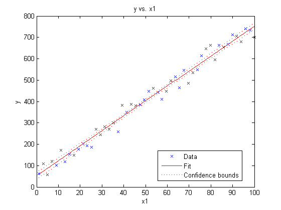
Notice that this simple command creates a plot with a wealth of information including
- A scatter plot of the original dataset
- A line showing our fit
- Confidence intervals for the fit
MATLAB has also automatically labelled our axes and added a legend.
Look for patterns in the residuals
Alternatively, lets assume that we wanted to see whether there was any pattern to the residuals. (A noticeable pattern to the residuals might suggest that our model is to simple and that it failed to capture a real work trend in the data set. This technique can also be used to check and see whether the noise component is constant across the dataset).
Here, I'll pass "myFit" to the new "plotResiduals" method and tell plotResiduals to plot the residuals versus the fitted values.
figure
plotResiduals(myFit, 'fitted')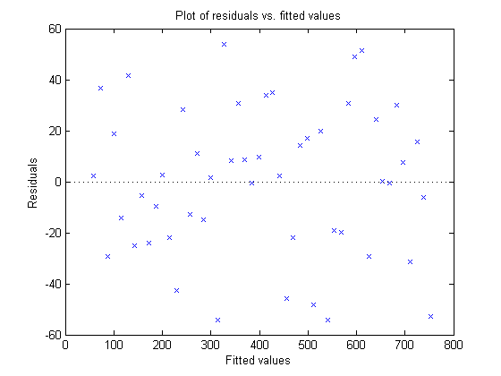
My plot looks like random noise - which in this case is a very good thing.
Look for autocorrelation in the residuals
Autocorrelation in my data set could also throw off the quality of my fit. The following command will modify the residual plot by plotting residuals versus lagged residuals.
figure
plotResiduals(myFit, 'lagged')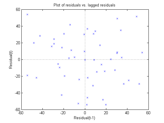
Look for outliers
Suppose that I wanted to check for outliers... We also have a plot for that.
figure
plotDiagnostics(myFit, 'cookd')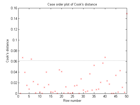
Cook's Distance is a metric that is commonly used to see whether a dataset contains any outliers. For any given data point, Cook's Distance is calculated by performing a brand new regression that excludes that data point. Cook's distance measures how much the shape of the curve changes between the two fits. If the curve moves by a large amount, that data point has a great deal of influence on the model and might very well be an outlier.
- The red crosses show the Cook's Distance for each point in the data set.
- The horizontal line shows "Three times the average Cook's Distance for all the points in the data set". Data points whose Cook's Distance is greater than three times the mean are often considered possible outliers.
In this example, non of our data points look as if they are outliers.
Use the resulting model for prediction
Last, but not least, lets assume that we wanted to use our model for prediction. This is as easy as applying the "predict" method.
Predictions = predict(myFit, New_X)
Predictions =
       310.51
       596.17
       64.866
       490.79
       306.06
       308.87
       621.55
       366.15
       543.32
       317.33
Discover the full set of methods available with regression objects
I hope that you agree that all these built in plots and analysis routines represent a significant improvement in usability. However, if you're anything like me, you immediate reaction is going to be "Great, you've built a lot of nice stuff, however, how do you expect me to find out about this?"
What I'd like to do now is show you a couple of simple tricks that you can use to discover all the new cabilities that we've added. The first trick is to recognize that "myFit" is an object and that objects have methods associated with them. All of the commands that we've sued so far like "plot", "plotResiduals", and "predict" are methods for the LinearModel object.
Any time that I'm working with one of the built in objects that ship with MATLAB my first plot is to inspect the full set of methods that ship with that object. This is as easy as typing methods(myFit) at the command line. I can use this to immediately discover all the built in capabilities that ship with the object. If one of those options catches my eye, I can use the help system to get more information.
methods(myFit)
Methods for class LinearModel:

addTerms              plot                  plotSlice
anova                 plotAdded             predict
coefCI                plotAdjustedResponse  random
coefTest              plotDiagnostics       removeTerms
disp                  plotEffects           step
dwtest                plotInteraction
feval                 plotResiduals

Static methods:

fit                   stepwise
Discover the full set of information included in the regression object
Here's another really useful trick to learn about the new regression objects. You can use the MATLAB variable editor to walk through the object and see all the information that is availabe.
You should have an object named "myFit" in the MATLAB workspace. Double clicking on the object will open the object in the Variable Editor.
Formulas
At the start of this blog there was some brief introduction to "formulas". I'd like to conclude this talk by providing a bit more information about formulas. Regression analysis requires the ability to specify a model that describes the relationship between your predictors and your response variables.
Let's change our initial example such that we're working with a high order polynomial rather than a straight line. I'm also going to change this from a curve fitting problem to a surface fitting problem.
X1 = 100 * randn(100,1);
X2 = 100 * rand(100,1);
X = [X1, X2];
Y = 3*X1.^2 + 5*X1.*X2 + 7* X2.^2 + 9*X1 + 11*X2 + 30 + 100*randn(100,1);
myFit2 = LinearModel.fit(X,Y)
myFit2 =
Linear regression model:
    y ~ 1 + x1 + x2

Estimated Coefficients:
                   Estimate    SE       tStat     pValue
    (Intercept)     25771      11230    2.2949     0.023893
    x1             178.75      54.95     3.253    0.0015717
    x2             613.39      187.2    3.2767    0.0014579

Number of observations: 100, Error degrees of freedom: 97
Root Mean Squared Error: 5.42e+04
R-squared: 0.211,  Adjusted R-Squared 0.195
F-statistic vs. constant model: 13, p-value = 1.03e-05
Let's take a look at the output from this example. We can see, almost immediately, that something has gone wrong with our fit.
- The R^2 value is pretty bad
- The regression coefficients are nowhere near the ones we specified when we created the dataset
If we look at the line that describes the linear regression model we can see what went wrong. By default, LinearModel will fit a plane to the dataset. Here, the relationship between X and Y is modelled as a high order polynomial. We need to pass this additional piece of information to "LinearModel".
Modeling a high order polynomial (Option 1)
Here are a couple different ways that I can use LinearModel to model a high order polynomial. The first option is to write out the formula by hand.
myFit2 = LinearModel.fit(X,Y, 'y ~ 1 + x1^2 + x2^2 + x1:x2 + x1 + x2')myFit2 =
Linear regression model:
y ~ 1 + x1*x2 + x1^2 + x2^2
Estimated Coefficients:
Estimate SE tStat pValue
(Intercept) 32.317 38.071 0.84886 0.39811
x1 9.1735 0.2119 43.291 6.9346e-64
x2 12.19 1.6568 7.3577 6.9388e-11
x1:x2 4.9985 0.0033943 1472.6 7.0691e-207
x1^2 2.9992 0.0006268 4785 5.5265e-255
x2^2 6.9849 0.015281 457.11 3.9814e-159
Number of observations: 100, Error degrees of freedom: 94
Root Mean Squared Error: 101
R-squared: 1, Adjusted R-Squared 1
F-statistic vs. constant model: 7.02e+06, p-value = 3.23e-260
Modeling a high order polynomial (Option 2)
Alternatively, I can simple use the the string "poly22" to indicate a second order polynomial for both X1 and X2 an automatically generate all the appropriate terms and cross terms.
myFit2 = LinearModel.fit(X, Y, 'poly22')myFit2 =
Linear regression model:
y ~ 1 + x1^2 + x1*x2 + x2^2
Estimated Coefficients:
Estimate SE tStat pValue
(Intercept) 32.317 38.071 0.84886 0.39811
x1 9.1735 0.2119 43.291 6.9346e-64
x2 12.19 1.6568 7.3577 6.9388e-11
x1^2 2.9992 0.0006268 4785 5.5265e-255
x1:x2 4.9985 0.0033943 1472.6 7.0691e-207
x2^2 6.9849 0.015281 457.11 3.9814e-159
Number of observations: 100, Error degrees of freedom: 94
Root Mean Squared Error: 101
R-squared: 1, Adjusted R-Squared 1
F-statistic vs. constant model: 7.02e+06, p-value = 3.23e-260
Nonlinear regression: Generate our data
Let's consider a nonlinear regression example. This time around, we'll work with a sin curve. The equation for a sin curve is governed by four key parameters.
- The phase
- The amplitude
- The vertical shift
- The phase shift
We'll start by generating a our dataset
X = linspace(0, 6*pi, 90);
X = X';
Y = 10 + 3*(sin(1*X + 5)) + .2*randn(90,1);
Nonlinear regression: Generate a fit
Next we'll using the NonLinearModel function to perform a nonlinear regression. Here we need to
- Specify formula that describes the relationship between X and Y
- Provide some reasonable starting conditions for the optimization solvers
myFit3 = NonLinearModel.fit(X,Y, 'y ~ b0 + b1*sin(b2*x + b3)', [11, 2.5, 1.1, 5.5])myFit3 =
Nonlinear regression model:
y ~ b0 + b1*sin(b2*x + b3)
Estimated Coefficients:
Estimate SE tStat pValue
b0 9.9751 0.02469 404.02 9.0543e-143
b1 2.9629 0.033784 87.703 6.4929e-86
b2 0.99787 0.0021908 455.47 3.029e-147
b3 5.0141 0.023119 216.88 1.4749e-119
Number of observations: 90, Error degrees of freedom: 86
Root Mean Squared Error: 0.227
R-Squared: 0.989, Adjusted R-Squared 0.989
F-statistic vs. constant model: 2.58e+03, p-value = 4.36e-84
Nonlinear regression: Work with the resulting model
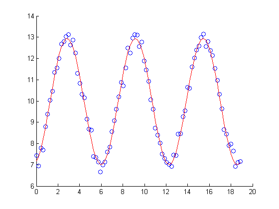
Once again, the output from the regression analysis is an object which we can used for analysis. For example:
figure
scatter(X,Y)
hold on
plot(X, myFit3.Fitted, 'r')
Nonlinear regression: Alternative ways to specify the regression model
One last point to be aware of: The syntax that I have been using to specify regression models is based on "Wilkinson's notation". This is a standard syntax that is commonly used in Statistics. If you prefer, you also have the option to specify your model using anonymous functions.
For example, that command could have been written as
myFit4 = NonLinearModel.fit(X,Y, @(b,x)(b(1) + b(2)*sin(b(3)*x + b(4))), [11, 2.5, 1.1, 5.5])
myFit4 =
Nonlinear regression model:
    y ~ (b1 + b2*sin(b3*x + b4))

Estimated Coefficients:
          Estimate    SE           tStat     pValue
    b1     9.9751       0.02469    404.02    9.0543e-143
    b2     2.9629      0.033784    87.703     6.4929e-86
    b3    0.99787     0.0021908    455.47     3.029e-147
    b4     5.0141      0.023119    216.88    1.4749e-119

Number of observations: 90, Error degrees of freedom: 86
Root Mean Squared Error: 0.227
R-Squared: 0.989,  Adjusted R-Squared 0.989
F-statistic vs. constant model: 2.58e+03, p-value = 4.36e-84
Conclusion
I've been working with Statistics Toolbox for close to five years now. Other than the introduction of dataset arrays a few years back, nothing has gotten me nearly as excited as the release of these new regression capabilities. So, it seemed fitting to conclude with an example that combines dataset arrays and the new regression objects.
Tell me what you think is going on in the following example. (Extra credit if you can work in the expression "dummy variable")
load carsmall

ds = dataset(MPG,Weight);
ds.Year = ordinal(Model_Year);

mdl = LinearModel.fit(ds,'MPG ~ Year + Weight^2')
mdl =
Linear regression model:
    MPG ~ 1 + Weight + Year + Weight^2

Estimated Coefficients:
                   Estimate      SE            tStat      pValue
    (Intercept)        54.206        4.7117     11.505    2.6648e-19
    Weight          -0.016404     0.0031249    -5.2493    1.0283e-06
    Year_76            2.0887       0.71491     2.9215     0.0044137
    Year_82            8.1864       0.81531     10.041    2.6364e-16
    Weight^2       1.5573e-06    4.9454e-07      3.149     0.0022303

Number of observations: 94, Error degrees of freedom: 89
Root Mean Squared Error: 2.78
R-squared: 0.885,  Adjusted R-Squared 0.88
F-statistic vs. constant model: 172, p-value = 5.52e-41
Post your answers here.




评论
要发表评论,请点击 此处 登录到您的 MathWorks 帐户或创建一个新帐户。