
Building Optimized Models in a few steps with AutoML
or: Optimized Machine Learning without the expertise
Today I'd like to introduce Bernhard Suhm who works as Product Manager for Machine Learning here at MathWorks. Prior to joining MathWorks Bernhard led analyst teams and developed methods applying analytics to optimizing the delivery of customer service in call centers. In today's post, Bernhard discusses how obtaining optimized machine learning models gets a lot easier and faster by applying AutoML. Instead of requiring significant machine learning expertise and following a lengthy iterative optimization process, AutoML delivers good models in a few steps.
Software requirements: Executing this script requires MATLAB version R2020a.
Contents
What is AutoML?
Building good machine learning models is an iterative process (as shown in the figure below). Achieving good performance requires significant effort: choosing a model (and then choosing a different model), identifying and extracting features, and even adding more or better training data.
Even experienced machine learning experts know it’s a lot of trial and error to finally arrive at a performant machine learning model.
Today, I’m going to show you how you can use AutoML to automate one (or all) of the following phases.
- Identifying features that have predictive power yet are not redundant
- Reducing the feature set to avoid overfitting and (if your application requires) fit the model on hardware with limited power and memory
- Selecting the best model and tune its hyperparameters

Figure 1 above shows a typical machine learning workflow. The orange boxes represent the steps we will automate with AutoML, and the following example will walk through the process of automating the feature extraction, model selection, hyperparameter tuning, and feature selection steps.
Example Application: A Human Activity Classifier
We'll demonstrate AutoML using the task of distinguishing what kind of activity you are doing based on data obtained from the accelerometer in your mobile device. For this example, we are trying to distinguish five activities: standing, sitting, walking upstairs vs downstairs vs straight. Figure 2 below shows thThe classifier is processing buffers of 128 samples, representing 2.56 seconds of activity, and windowing overlaps the signal by half that. We'll use a training set comprising of 25 subjects and 6873 observations, and a test set comprising of 5 subjects and about 600 observations.

Let's first prepare our workshop and load the example data.
warning off;
rng('default');
Load accelerometer data divided in training and test sets
load dataHumanActivity.mat
Get handle on number of samples
unbufferedCounts = groupcounts(unbufferedTrain,{'subject','activity'});
Now we are ready to discuss the three primarily steps of applying AutoML to signal and image data, and apply them to our human activity classification problem:
- Extract Initial features by applying Wavelet Scattering
- Automatically select a small subset of features
- Model selection and optimization
Step 1: Extract Initial Features Automatically by Applying Wavelet Scattering
Machine learning practitioners know obtaining good features can take a lot of time and be outright daunting for someone without the necessary domain knowledge, like with signal processing. AutoML provides feature generation methods that automatically extract high performing features from sensor and image data. One such method is Wavelet scattering which derives, with minimal configuration, low-variance features from signal (and image) data for use in machine learning and deep learning application.
You don't need to understand Wavelet scattering to successfully apply it, but in brief, Wavelets transform small deformations in the signal by separating the variations across different scales. For many natural signals, the wavelet transform also provides a sparse representation. It turns out the filters in the initial layers of fully trained deep networks resemble wavelet like filters. The wavelet scattering network represents such a set of pre-defined filters.
To apply Wavelet scattering you only need the sample frequency, the minimum number of samples across the buffers in your data set, and a function that applies the Wavelet transformation using built-in function featureMatrix across a set of signal data. We included one way to do so in the appendix; or as an alternative you can apply featureMatrix across a datastore.
N =  min(unbufferedCounts.GroupCount);
sf = waveletScattering('SignalLength',N, 'SamplingFrequency',50);

trainWavFeatures = extractFeatures(unbufferedTrain,sf,N);
testWavFeatures = extractFeatures(unbufferedTest,sf,N);
On this human activity data, we obtain 468 wavelet features - quite many - but automated feature selection will help us pare them down.
Step 2: Automated Feature Selection
Feature selection is typically used for the following two main reasons:
- Reduce the size of a large models so they fit on memory (and power) constrained embedded devices
- Prevent overfitting
Since wavelet scattering typically extracts hundreds of features from the signal or image, the need to reduce them to a smaller number is more pressing than with a few dozen manually engineered features.
Many methods are available to automatically select features. Here is a comprehensive overview what's available in MATLAB. Based on experience, Neighborhood Component Analysis (fscnca) and Maximum Relevance Minimum Redundancy (fscmrmr) deliver good results with limited runtime. Let's apply MRMR to our human activity data and plot the first 50 ranked features:
[mrmrFeatures , scores] = fscmrmr(trainWavFeatures, 'activity');

stem(scores(mrmrFeatures(1:50)),'bo');

Once we have all the features ranked, we need to decide how many predictors to use. Turns out a fairly low number of the Wavelet features provide good performance. For this example, to be able to compare the performance of the model obtained with AutoML to previous versions of the human activity classifier, we pick the same number that we selected leaving out low variance features from the >60 manually engineered ones. Optimizing accuracy on cross validation suggests a modestly higher number of features between 16 and 28, depending on which feature selection method you apply.
topFeaturesMRMR = mrmrFeatures(1:14);
Step 3: Obtain Optimized Model In One-Step
There is no one-size fits all in machine learning - you need to try out multiple models to find a performant one. Further, optimal performance requires careful tuning of hyperparameters that control the algorithm’s behavior. Manual hyperparameter tuning requires expert experience, rules of thumb, or brute-force search of numerous parameter combinations. Automated hyperparameter tuning makes it easy to find the best settings, and computational burden can be minimized by applying Bayesian optimization. Bayesian optimization internally maintains a surrogate model of the objective function, and in each iteration determines the most promising next parameter combination, balancing progressing towards an optimum that may be local with exploring areas that have not yet been evaluated.
Bayesian optimization can also be applied to identifying the type of model. Our new fitcauto function, which was released with R2020a, uses a meta-learning model to narrow the set of models that are considered. The meta-learning model identifies a small subset of candidate models that are well suited for a machine learning problem, given various characteristics of the features. A meta-learning heuristic was derived from publicly available datasets, for which pre-determined characteristics can be computed, and associated with a variety of models and their performance.
With fitcauto, identifying the best combination of model and optimized hyperparameters essentially becomes a one liner, aside from defining some basic parameters controlling execution, like limiting the number of iterations to 50 (to keep runtime to a few minutes).
opts = struct('MaxObjectiveEvaluations',50, 'ShowPlots',true);
modelAuto = fitcauto(trainWavFeatures(:,topFeaturesMRMR),...
    trainWavFeatures.activity,'Learners','all',...
    'HyperparameterOptimizationOptions',opts);
|====================================================================================================================| | Iter | Eval | Objective | Objective | BestSoFar | BestSoFar | Learner | Hyperparameter: Value | | | result | | runtime | (observed) | (estim.) | | | |====================================================================================================================| | 1 | Best | 0.10489 | 5.4013 | 0.10489 | 0.10489 | ensemble | Method: RUSBoost | | | | | | | | | NumLearningCycles: 87 | | | | | | | | | LearnRate: 0.88361 | | | | | | | | | MinLeafSize: 14 | | 2 | Accept | 0.15733 | 0.064101 | 0.10489 | 0.10489 | tree | MinLeafSize: 147 | | 3 | Accept | 0.16178 | 0.071101 | 0.10489 | 0.10489 | knn | NumNeighbors: 8 | | | | | | | | | Distance: correlation | | 4 | Best | 0.056 | 0.077703 | 0.056 | 0.10489 | nb | DistributionNames: normal | | | | | | | | | Width: NaN | | 5 | Accept | 0.31822 | 178.04 | 0.056 | 0.10489 | svm | Coding: onevsall | | | | | | | | | BoxConstraint: 881.45 | | | | | | | | | KernelScale: 0.052695 | | 6 | Accept | 0.072 | 1.3751 | 0.056 | 0.0648 | nb | DistributionNames: kernel | | | | | | | | | Width: 0.013961 | | 7 | Accept | 0.10667 | 0.073527 | 0.056 | 0.0648 | discr | Delta: 1.0971 | | | | | | | | | Gamma: 0.26706 | | 8 | Accept | 0.6 | 0.062479 | 0.056 | 0.0648 | discr | Delta: 8.1232 | | | | | | | | | Gamma: 0.69599 | | 9 | Accept | 0.096 | 16.472 | 0.056 | 0.0648 | ensemble | Method: RUSBoost | | | | | | | | | NumLearningCycles: 290 | | | | | | | | | LearnRate: 0.0054186 | | | | | | | | | MinLeafSize: 9 | | 10 | Accept | 0.058667 | 0.062727 | 0.056 | 0.0648 | discr | Delta: 0.0010027 | | | | | | | | | Gamma: 0.91826 | | 11 | Accept | 0.067556 | 0.080417 | 0.056 | 0.0648 | tree | MinLeafSize: 3 | | 12 | Accept | 0.8 | 0.061978 | 0.056 | 0.0648 | discr | Delta: 316.68 | | | | | | | | | Gamma: 0.97966 | | 13 | Accept | 0.46844 | 0.35913 | 0.056 | 0.0648 | svm | Coding: onevsall | | | | | | | | | BoxConstraint: 0.001978 | | | | | | | | | KernelScale: 3.4614 | | 14 | Accept | 0.10844 | 0.072236 | 0.056 | 0.0648 | tree | MinLeafSize: 17 | | 15 | Accept | 0.056 | 0.074398 | 0.056 | 0.060053 | nb | DistributionNames: normal | | | | | | | | | Width: NaN | | 16 | Accept | 0.056889 | 0.06201 | 0.056 | 0.060053 | discr | Delta: 0.00061575 | | | | | | | | | Gamma: 0.81629 | | 17 | Accept | 0.8 | 0.06456 | 0.056 | 0.060053 | knn | NumNeighbors: 2 | | | | | | | | | Distance: jaccard | | 18 | Accept | 0.11111 | 0.070893 | 0.056 | 0.060053 | tree | MinLeafSize: 19 | | 19 | Accept | 0.49511 | 0.098951 | 0.056 | 0.060053 | knn | NumNeighbors: 544 | | | | | | | | | Distance: minkowski | | 20 | Accept | 0.094222 | 0.066813 | 0.056 | 0.060053 | knn | NumNeighbors: 10 | | | | | | | | | Distance: cosine | |====================================================================================================================| | Iter | Eval | Objective | Objective | BestSoFar | BestSoFar | Learner | Hyperparameter: Value | | | result | | runtime | (observed) | (estim.) | | | |====================================================================================================================| | 21 | Accept | 0.061333 | 10.548 | 0.056 | 0.060053 | svm | Coding: onevsall | | | | | | | | | BoxConstraint: 298.57 | | | | | | | | | KernelScale: 1.4571 | | 22 | Accept | 0.8 | 0.074188 | 0.056 | 0.060053 | discr | Delta: 92.633 | | | | | | | | | Gamma: 0.48063 | | 23 | Accept | 0.090667 | 0.92212 | 0.056 | 0.060053 | ensemble | Method: AdaBoostM2 | | | | | | | | | NumLearningCycles: 17 | | | | | | | | | LearnRate: 0.0013648 | | | | | | | | | MinLeafSize: 5 | | 24 | Accept | 0.11111 | 0.098575 | 0.056 | 0.060053 | tree | MinLeafSize: 57 | | 25 | Accept | 0.056 | 0.080269 | 0.056 | 0.0604 | nb | DistributionNames: normal | | | | | | | | | Width: NaN | | 26 | Accept | 0.14222 | 0.54873 | 0.056 | 0.0604 | svm | Coding: onevsone | | | | | | | | | BoxConstraint: 148.79 | | | | | | | | | KernelScale: 27.357 | | 27 | Accept | 0.10222 | 1.0631 | 0.056 | 0.0604 | ensemble | Method: AdaBoostM2 | | | | | | | | | NumLearningCycles: 20 | | | | | | | | | LearnRate: 0.02154 | | | | | | | | | MinLeafSize: 109 | | 28 | Accept | 0.6 | 3.1074 | 0.056 | 0.0604 | ensemble | Method: AdaBoostM2 | | | | | | | | | NumLearningCycles: 83 | | | | | | | | | LearnRate: 0.0038432 | | | | | | | | | MinLeafSize: 412 | | 29 | Accept | 0.11022 | 0.41982 | 0.056 | 0.0604 | svm | Coding: onevsone | | | | | | | | | BoxConstraint: 0.8938 | | | | | | | | | KernelScale: 1.2517 | | 30 | Accept | 0.056889 | 0.064237 | 0.056 | 0.0604 | discr | Delta: 4.0389e-06 | | | | | | | | | Gamma: 0.7838 | | 31 | Accept | 0.6 | 0.97945 | 0.056 | 0.0604 | ensemble | Method: AdaBoostM2 | | | | | | | | | NumLearningCycles: 25 | | | | | | | | | LearnRate: 0.005856 | | | | | | | | | MinLeafSize: 391 | | 32 | Best | 0.027556 | 1.4236 | 0.027556 | 0.0604 | svm | Coding: onevsone | | | | | | | | | BoxConstraint: 568.53 | | | | | | | | | KernelScale: 2.5259 | | 33 | Accept | 0.10222 | 0.071448 | 0.027556 | 0.0604 | tree | MinLeafSize: 16 | | 34 | Accept | 0.058667 | 0.06672 | 0.027556 | 0.0604 | discr | Delta: 5.6703e-06 | | | | | | | | | Gamma: 0.0022725 | | 35 | Accept | 0.072889 | 1.2183 | 0.027556 | 0.0604 | ensemble | Method: AdaBoostM2 | | | | | | | | | NumLearningCycles: 24 | | | | | | | | | LearnRate: 0.026186 | | | | | | | | | MinLeafSize: 36 | | 36 | Accept | 0.078222 | 0.075859 | 0.027556 | 0.0604 | tree | MinLeafSize: 7 | | 37 | Accept | 0.056889 | 0.063344 | 0.027556 | 0.0604 | discr | Delta: 0.00043899 | | | | | | | | | Gamma: 0.72219 | | 38 | Accept | 0.23644 | 0.92978 | 0.027556 | 0.10559 | nb | DistributionNames: kernel | | | | | | | | | Width: 0.0018864 | | 39 | Accept | 0.45867 | 180.44 | 0.027556 | 0.10559 | svm | Coding: onevsall | | | | | | | | | BoxConstraint: 122.06 | | | | | | | | | KernelScale: 0.013471 | | 40 | Accept | 0.072 | 0.063096 | 0.027556 | 0.10559 | knn | NumNeighbors: 4 | | | | | | | | | Distance: cosine | |====================================================================================================================| | Iter | Eval | Objective | Objective | BestSoFar | BestSoFar | Learner | Hyperparameter: Value | | | result | | runtime | (observed) | (estim.) | | | |====================================================================================================================| | 41 | Accept | 0.10756 | 0.073934 | 0.027556 | 0.10611 | tree | MinLeafSize: 41 | | 42 | Accept | 0.35111 | 1.242 | 0.027556 | 0.10611 | nb | DistributionNames: kernel | | | | | | | | | Width: 10.9 | | 43 | Accept | 0.058667 | 0.064954 | 0.027556 | 0.10611 | discr | Delta: 0.011214 | | | | | | | | | Gamma: 0.626 | | 44 | Accept | 0.056 | 0.075895 | 0.027556 | 0.10611 | nb | DistributionNames: normal | | | | | | | | | Width: NaN | | 45 | Accept | 0.68444 | 0.86246 | 0.027556 | 0.10611 | nb | DistributionNames: kernel | | | | | | | | | Width: 0.00020857 | | 46 | Accept | 0.8 | 0.085589 | 0.027556 | 0.10611 | knn | NumNeighbors: 543 | | | | | | | | | Distance: jaccard | | 47 | Accept | 0.056889 | 0.063729 | 0.027556 | 0.10611 | discr | Delta: 2.2103e-05 | | | | | | | | | Gamma: 0.73064 | | 48 | Accept | 0.099556 | 0.073035 | 0.027556 | 0.10611 | knn | NumNeighbors: 11 | | | | | | | | | Distance: euclidean | | 49 | Accept | 0.21156 | 0.12333 | 0.027556 | 0.10611 | knn | NumNeighbors: 74 | | | | | | | | | Distance: mahalanobis | | 50 | Accept | 0.056 | 0.076537 | 0.027556 | 0.10611 | nb | DistributionNames: normal | | | | | | | | | Width: NaN | __________________________________________________________ Optimization completed. MaxObjectiveEvaluations of 50 reached. Total function evaluations: 50 Total elapsed time: 554.4276 seconds. Total objective function evaluation time: 407.7031 Best observed feasible point is a multiclass svm model with: Coding (ECOC): onevsone BoxConstraint: 568.53 KernelScale: 2.5259 Observed objective function value = 0.027556 Estimated objective function value = 0.21986 Function evaluation time = 1.4236 Best estimated feasible point (according to models) is a tree model with: MinLeafSize: 147 Estimated objective function value = 0.10611 Estimated function evaluation time = 0.075541


After 50 iterations, the best performing model on this data set is an Ada-boosted decision tree, which achieves with just 14 features 99% accuracy on held-out test data. That compares favorably to the best models you can obtain with manually engineered features and model tuning!
predictionAuto = predict(modelAuto, testWavFeatures);
accuracy = 100*sum(testWavFeatures.activity == predictionAuto)/size(testWavFeatures,1);
round(accuracy)
ans =
    88
Summary
In summary, we have described an approach that reduces building effective machine learning models for signal and image classification tasks to three simple steps: automatically extract features by applying wavelet scattering technique; second, automated feature selection that identifies a small subset of features with little loss in accuracy; and third, automatically selecting and optimizing a model whose performance gets close to that of models manually optimized by skilled data scientists. AutoML empowers practitioners with little to no expertise in machine learning to obtain models that achieve near-optimal performance.
This article just provided a high-level overview of what AutoML is available in MATLAB today. Being the product manager of the Statistics and Machine Learning Toolbox. I’m always curious to hear your use cases and expectations you have for for AutoML. Here's some resources for you to explore.
- Learn more about AutoML here
- Try it out by extending our heart sound classifier demo to use fitcauto to find a good model
And please leave a comment here to share your thoughts.
Appendix: Wavelet scattering function
Here's the function that applies wavelet scattering over a buffer of signal data.
function featureT = extractFeatures(rawData, scatterFct, N)
% EXTRACTFEATURES.M - Apply wavelet scattering to raw data  (3 dimensional
% signal plus "activity" label), using scatterFct on signal of length N

% extract X, Y, Z from raw data (columns 2-4), and sort by subject
signalData = table2array(rawData(:,2:4));
[gTrain, ~,activityTrain] = findgroups(rawData.subject, rawData.activity);

% Apply wavelet scattering featureMatrix on all rows from each subject.
% We get back 3-dimensional matrices (#features, #time-intervals, 3 signals)
waveletMatrix = splitapply(@(x) {featureMatrix(scatterFct,(x(1:N,:)))},signalData,gTrain);

featureT = table;    % feature table we'll build up

% loop over each of the Wavelet matrices that were created above
for i = 1 : size(waveletMatrix,1)

    oneO = waveletMatrix{i};   % process this observation
    thisObservation = [oneO(:,:,1); oneO(:,:,2); oneO(:,:,3)];
    thisObservation = array2table(thisObservation');  % don't forget to convert the features from rows into columns

    featureT = [featureT; thisObservation];
end

% get labels by duplicating label for each row of "wavelet" features obtained for  subject x activity
featureT.activity = repelem(activityTrain,size(waveletMatrix{1},2));

end


댓글
댓글을 남기려면 링크 를 클릭하여 MathWorks 계정에 로그인하거나 계정을 새로 만드십시오.