
How to Win at Formula SAE using Simulink
Todays guest bloggers are Erin, Matt, Kattly, Greg, and Andrew of the McGill Formula Electric team at McGill University in Montreal, Canada. They’ll explain their success story and why simulation was key to their success. Also learn from them why it is good to struggle, fall and then get up again. Following the great community spirit within Formula Student, Erin and the team also open-sourced most of their work, find it on MATLAB Central FileExchange and linked here in the post.
—
Introduction
In recent years, we’ve seen running simulations and building control systems become more and more crucial for any trophy winning FSAE car, but for our team these projects seemed undefined. To start simple, we spent the past year researching and designing a few basic control systems and simulations for our rear-wheel drive vehicle that we could build and run in Simulink; we built a point-mass vehicle model, a longitudinal traction control system, a lap sim, and a quarter car ride model. While our team goals for this year were to produce a reliable, serviceable, and light car, our additional controls/vehicle dynamics goal was to focus on getting comfortable with the Simulink systems we were building in preparation for competition and for the following year. With these, we brought home first place at FSAE Lincoln and are excited to write a torque vectoring algorithm, a two-track vehicle model, and a full ride model for our newly all-wheel drive car in the coming year.
Traction Controller Design
Vehicle Model
We chose a design methodology for the vehicle model that would provide adequate simulation accuracy without being too resource intensive to design. We realized that by starting with a simple point mass model and adding known efficiencies and losses we could come very close to what we observed on track.
Our model consists of a vehicle body and a drivetrain system. The vehicle body represents the point mass and contains load transfer and aerodynamic calculations. The drivetrain includes our motor, gearing, differential, and tire model. Many of the components require only simple physics to initially get results. Once the basics work, efficiencies, losses, and more advanced modelling can be added as required to get the simulation to match testing data.
The most difficult part of making the vehicle model was integrating the tire model. We ended up using MFeval, which is a free library available on the MATLAB file exchange, to do this. MFeval contains the necessary equations to evaluate magic formula models from TIR files.
Finally, we needed to validate the model so that it could reliably be used to tune traction control. We used testing data from past years to determine if the acceleration, wheel speeds, and slip response from our model matched a real acceleration test. We fed the model the logged throttle input and analyzed how its output matched the logged vehicle response. After some tuning and adjustment of correction values, we had a model which approximated our car’s longitudinal behavior.
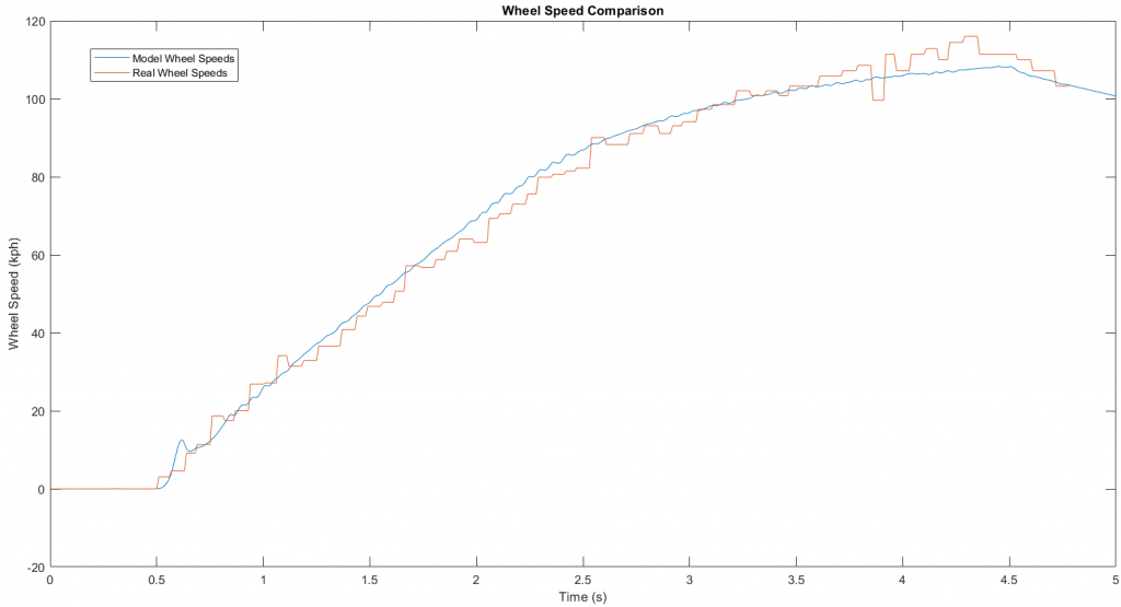
MATLAB graph showing the comparison between the rear wheel speeds from a real acceleration run (orange) and the model’s output in blue. The acceleration, top speed and slip characteristics all match very closely.
Traction Controller
Our longitudinal traction control system was then built, tuned, and deployed to our custom vehicle controller using Simulink. It consists of a vehicle state estimator which calculates axle speeds and a forward torque controller which prevents vehicle slip to improve acceleration times.
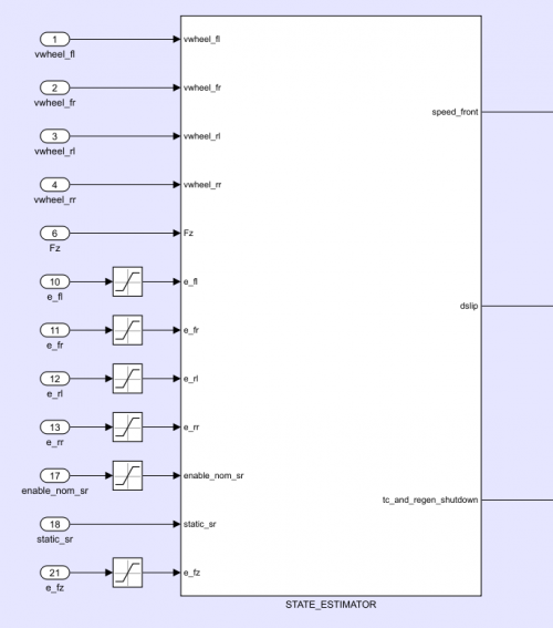
State Estimator calculates axle speeds and the delta between target and real slip ratios (dslip); outputs are fed into forward torque controller
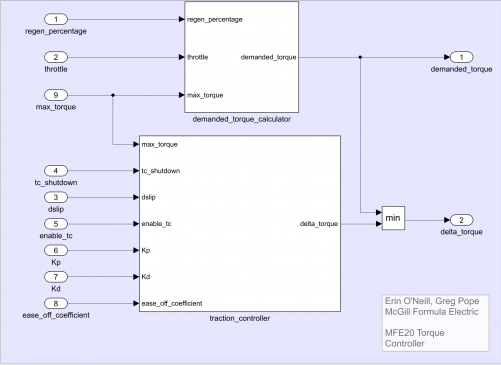
Forward torque controller calculates driver demanded torque and the torque by
which it should be decreased in order to keep dslip less than or equal to 0
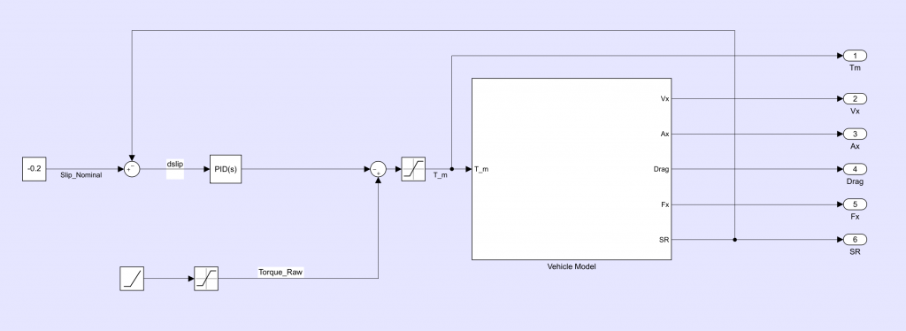
In order to streamline on-track testing we used the vehicle model to tune different traction control ‘modes’ which were then toggled with a button on the dash (and would input different gains into the traction controller). To find these 10 modes, we hooked our PID controller up to the vehicle model and tuned it for different responses ranging from conservative to aggressive. We were then able to quickly test these by toggling the modes from the dash and adjusting them offline, all of which helped to increase the efficiency of on-track time.
Once we had the model built, we then had to get it running on the car. At first, it seemed like there was a lot of conflicting information online about this process. We followed the MATLAB documentation regarding C-Code Generation for Models and it made generating code from our Simulink model very straightforward.
After getting the C files we had to figure out how to incorporate them into our vehicle controller’s code; we use the NXP MPC5744p MCU on a custom PCB for our vehicle controller. The code interface report that Simulink generates documents the 4 main APIs that you need to call in order to interact with your new C ‘library:’
- The first function is basically a constructor that gives you a data structure you use to interact with the model.
- The second function initializes the data structure that you got from step 1.
- Then you can interact with the Simulink generated code by setting inputs in the data structure’s ‘inputs’ field and reading outputs from its ‘outputs’ field. Whenever you want to iterate through one step of the Simulink model, set all the appropriate inputs and call the provided ‘Step’ function, after which you can retrieve the outputs from the data structure as mentioned before.
- When you’re done with the Simulink model, call the terminate function and it will clean everything up for you.
The whole process from running the torque controller in Simulink to running it on our board probably took us about 30 minutes to set up and now takes about 3 minutes to update if we change the Simulink model.
With this simple Simulink model running on our car we were able to decrease our acceleration time at Lincoln by almost half a second! To show this, below we have some plots from two of our acceleration runs at Lincoln, one using and one not using traction control.
Lincoln acceleration run without traction control, 4.16s:
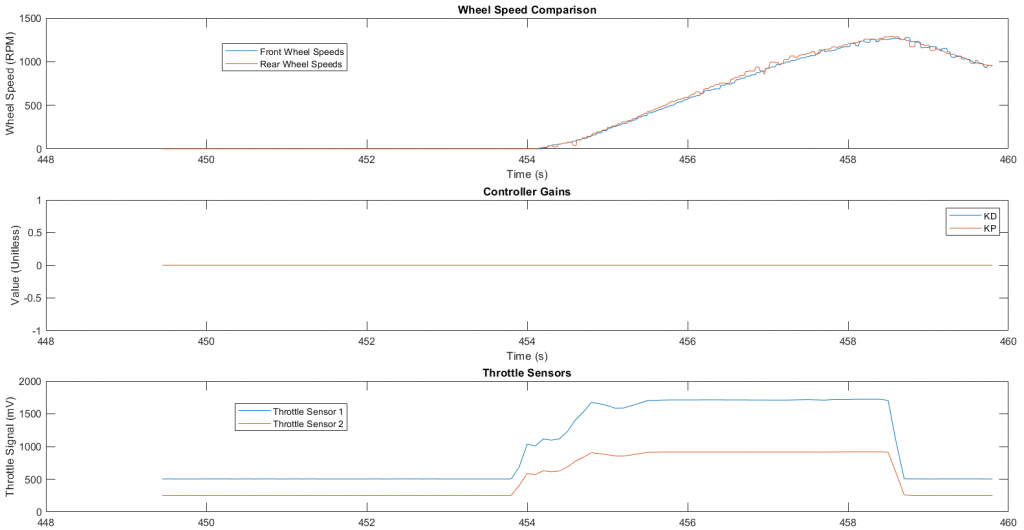
At first our results seemed a bit surprising; even though traction control was not applied, we see that the driver wasn’t slipping. Considering the track was wet for our accel runs and our main goal was to maintain traction, we looked at the throttle to see what the driver was doing to achieve this. He was controlling slip by very carefully applying the throttle: see how long it took him to reach full throttle and how careful his approach to it was. Our next run, however, we turned traction control on, and this time the driver didn’t have to control slip by carefully limiting throttle. Instead he was able to reach maximum throttle position almost immediately while our Simulink model did the rest.
Lincoln acceleration with traction control, 3.687s:
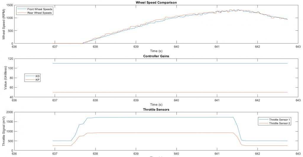
This time the car reaches top speeds much faster! Because our Simulink model can control slip much faster than the driver could in the previous run, he reached full throttle much quicker than before and, therefore, we see that the car accelerates much faster with than without traction control.
Lap time Simulation
Creating a lap time simulation is very important for any FSAE team. We use it to get an idea of how different vehicle parameters affect our car’s performance in dynamic events. This helps to guide high-level design decisions such as motor selection, battery pack sizing, aero targets, gear ratio, vehicle mass targets, etc.
Previous Racing Lounge videos explain different approaches (ETH Zurich, TU Munich), both of which use a two-track car model with a tire model based on test data from the TTC or elsewhere. For simplicity, we decided to model the car as a point-mass and model the tires using a constant coefficient of friction. This simpler approach still gives us great insight into how high-level parameters affect the car. Our lap sim is quasi-steady state and works by dividing the track into segments, adding up the forces applied to the car at each point and dividing by mass to get the vehicle’s acceleration. It then uses a basic forward-Euler method to solve for the car’s velocity and displacement. This approach is widely used and there is lots of documentation about it online.

As with any simulation, it is important to validate and modify the model to correspond to data from the track. In order to validate the lap time simulation, it’s important to correlate the lap time sensitivities and the energy consumption from changing a parameter (like the change in lap time after adding 5kg), and to validate the lap time obtained by the model with data from the car on-track. A basic testing plan would look something like the following:
- Run the car in its normal configuration
- Run with 5kg of ballast added
- Run with no aero (or in a low drag configuration)
One thing to keep in mind is the consistency/skill of your drivers when validating your model. The lap time simulation is idealized, and most FSAE drivers are not racing drivers, so you will need to take that into account during the validation process.
Quarter Car Model for Suspension Setup
The ride model is a useful tool for optimizing spring and damper settings, characterizing ride quality, and analyzing handling. It was a new project we wanted to take on to improve our suspension setups and to further our understanding of our car’s dynamics.
The original goal was to get a 7DOF full ride model in Simulink and to input track data to simulate a full circuit. Given that this model was a team first, it was too ambitious, and we realized that to succeed we needed a full understanding of our fundamentals. We scaled back to a quarter car model, validated it, used it to justify parts of our design for next year, and are now building off it for a half car model before re-approaching the full ride model.
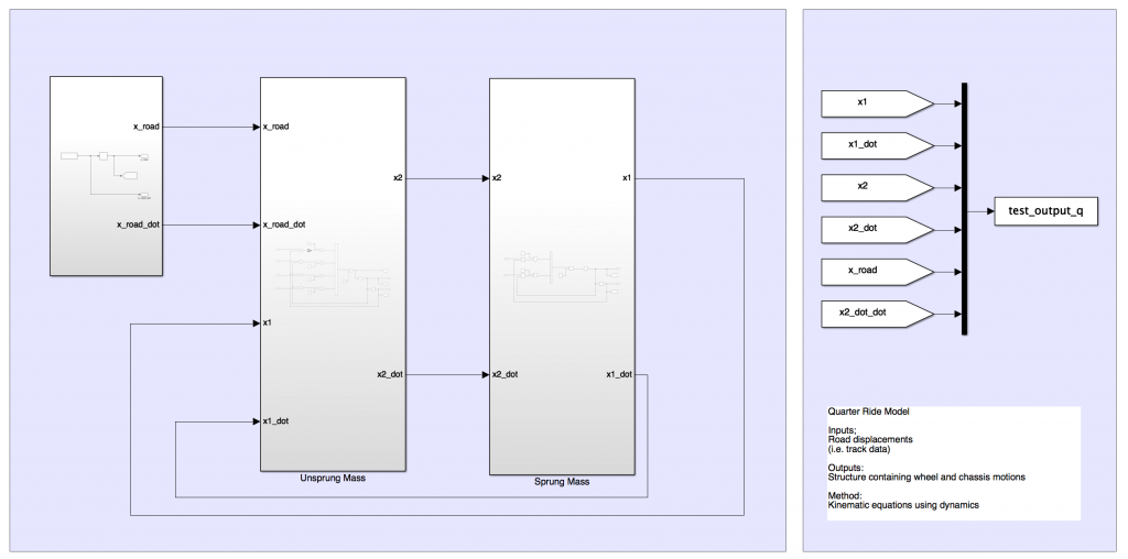
For the quarter car model, we used an equations-based approach in Simulink with outputs to MATLAB. It consists of three subsystems: road inputs, unsprung mass, and sprung mass. We validated our model by correlating the linear potentiometer data we logged from a step input to our car.
The outputs for chassis displacement from the Simulink model are very close to the actual displacements from our linpots; we used this to justify our damper force graphs during design at Lincoln. For next year, we are fully analyzing our suspension settings with the quarter car model and using it as a baseline to build our half car model. The half car model will enable ride quality modelling and will help us to maintain our aero targets.
This was a big learning year for us, but Simulink was a huge help in making our win at Lincoln possible; if you’re considering the move to more complicated vehicle dynamics and controls systems I think our entire team would say ‘take the leap!’ It will be a growth year, but Simulink allows you to focus on design so that you can be ready to present your work at comp and to take even bigger steps the following year!
Cheers!
Erin, Matt, Kattly, Greg, and Andrew
- Category:
- Automotive,
- Education,
- Simulink,
- Skills,
- Team achievements


Comments
To leave a comment, please click here to sign in to your MathWorks Account or create a new one.