In my August 7th post on upslope area, I showed how to construct and solve the flow matrix to determine the upslope area for every pixel in a digital elevation model (DEM). In addition, the flow matrix can be used to compute both the influence map and the dependence map.

The influence map shows where water starting from a particular pixel will drain. The dependence map shows which uphill pixels drain through a particular pixel. Let's look at how to compute these from the flow matrix.

Recall the form of the flow equation for a particular pixel: The upslope area of a pixel equals 1 plus a weighted fraction of the upslope area of each of its neighbors.

The 1 term comes from assuming each pixel contributes an equal volume to the overall flow across the terrain. Think of it as rain falling equally on each pixel. To compute the influence map, then, we just have to modify our set of equations so that the 1 term appears only for the pixel or pixels of interest. Fortunately, that only affects the right-hand side of the equation, not the flow matrix itself. So solving for the influence map a particular pixel looks almost like solving for upslope area for all pixels.

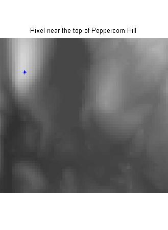
Here's an example from the Milford, Massachusetts DEM that I've used before:

s = load('milford_ma_dem');
E = s.Zc;
imshow(E, [])
limits = [160 220 215 270];
axis(limits);
hold on
plot(169, 227, '*')
hold off
title('Pixel near the top of Peppercorn Hill')

Find the flow directions and flow matrix using dem_flow and flow_matrix from my upslope area toolbox on MATLAB Central:

R = dem_flow(E);
T = flow_matrix(E, R);

Make a vector for the right-hand side that has a single 1 corresponding to the (227,169) pixel:

[M, N] = size(E);
rhs = zeros(numel(E), 1);
idx = (169-1)*M + 227;
rhs(idx) = 1;

Solve for the influence map:

I = T \ rhs;
I = reshape(I, M, N);
imshow(I,[])
axis(limits);
title('Influence map')

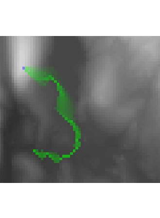
The influence_map function does all this for you. I also included a visualization function (vis_map) that superimposes the influence (or dependence) map transparently, in green, on top of the original DEM. The starting pixels are superimposed in blue. Here's what it looks like for our example:

vis_map(I, E, 227, 169);
axis(limits);

To compute the dependence map, you can't use the flow matrix exactly as is; you have to transpose it. Otherwise, it's very similar to the influence map computation. See the code in dependence_map for the details.

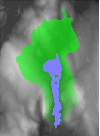
Here's an example that computes the dependence map for an entire set of pixels, not just a single pixel. Specifically, it's the dependence map for North Pond:

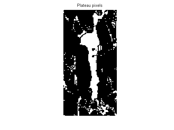
plateaus = imerode(E, ones(3, 3)) == E;
pond = bwselect(plateaus, 183, 170);
D = dependence_map(E, T, pond);
vis_map(D, E, pond);
xlim([110 240])
ylim([80 260])

Next time I plan to talk about vectorizing the pixel flow direction calculation.

Get the MATLAB code

Published with MATLAB® 7.5