Fourier transform visualization using windowing
When I dipped my toe into the Fourier transform waters last week, the resulting comments and e-mail indicated there is a lot of interest in tutorial material and explanations. I'm willing, but I'll have to think about how to do it. I haven't taught that material since my professor days, and that was many, many moons ago.
But I can certainly start by following up on the teaser example from last week. A reader of Digital Image Processing Using MATLAB wanted to know why the Fourier transform of the image below looked so "funny." (For the moment I'm going to use the term Fourier transform fairly loosely as many people do.)
url = 'https://blogs.mathworks.com/images/steve/2009/lines.png';
f = imread(url);
imshow(f)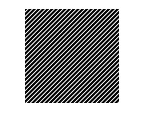
I didn't show what the Fourier transform looked like, though, so I suppose it wasn't very clear what problem I was talking about.
The book recommends this procedure for visualizing the Fourier transform of an image:
F = fft2(f);
imshow(log(abs(fftshift(F)) + 1), [])
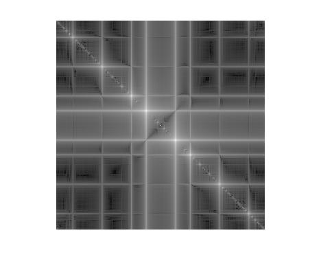
The puzzle is why does the Fourier transform look so complicated? The input image, after all, contains only a simple sinusoidal pattern.
The answer is related to the fact that what we're actually computing when we call fft2 is the two-dimensional discrete Fourier transform (DFT). The DFT has an implicit periodicity in both the spatial and the frequency domains. We don't often don't think about the periodicity in either domain, both because we only need one period for computation and because only one period is usually shown.
Let's see what happens when you take the original image and replicate it a few times.
I4 = repmat(I, 2, 2);
imshow(I4)
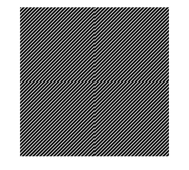
Suddenly the simple sinusoidal pattern doesn't look quite so simple. What you get here (besides eye strain from looking at this image) is a pattern of small vertical and horizontal discontinuities. These discontinuities are producing the rectangular pattern in the frequency-domain visualization above. That's because any kind of discontinuity has frequency-domain energy across a broad range of frequencies.
I see this kind of thing in Fourier transform plots all the time, although often the effect is more subtle. Here's another example.
g = imread('rice.png');
imshow(g)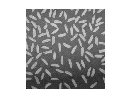
G = fft2(g);
imshow(log(abs(fftshift(G)) + 1), [])
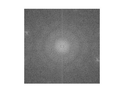
What's that vertical line in the frequency domain? There are no horizontal features in the image to account for it. At least, no horizontal features are apparent until you display the periodically replicated image.
imshow(repmat(g, 2, 2))
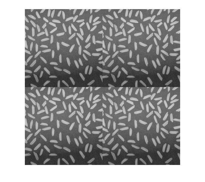
Since the original image is darker at the bottom than at the top, there is a strong horizontal discontinuity at the periodic boundary. That's what causes the vertical line to appear in the frequency domain.
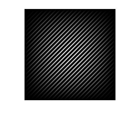
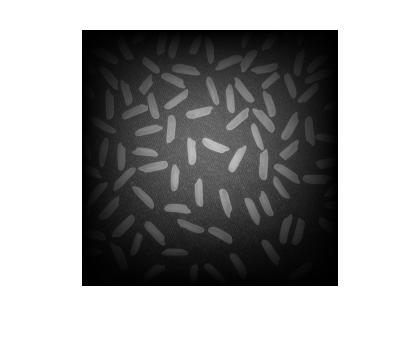
One way to remove these frequency-domain effects is to taper the original image values toward 0 at the image boundaries. That removes the periodic discontinuities. The tapering can be done by elementwise multiplication of the original image by a matrix equal to 1 in the center and trending toward 0 at the edges. This is called windowing.
Let's try that here using a raised cosine function.
[M, N] = size(f);
w1 = cos(linspace(-pi/2, pi/2, M));
w2 = cos(linspace(-pi/2, pi/2, N));
w = w1' * w2;
f2 = im2uint8(im2single(f) .* w);
imshow(f2)
F2 = fft2(f2);
imshow(log(abs(fftshift(F2)) + 1), [])
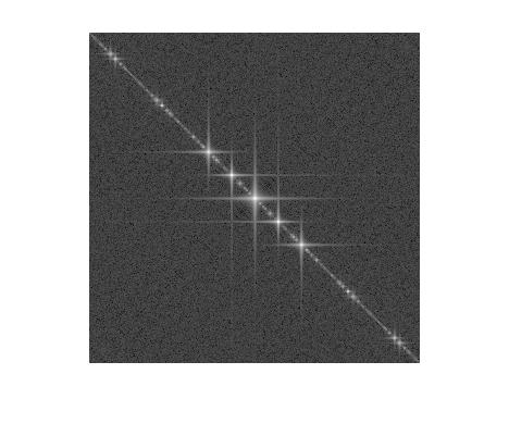
Although there are still some visible artifacts, this frequency-domain plot is much closer to showing what we might have expected: the Fourier transform of a simple sinusoidal pattern.
Here's the same procedure applied to the rice image.
[M, N] = size(g);
w1 = cos(linspace(-pi/2, pi/2, M));
w2 = cos(linspace(-pi/2, pi/2, N));
w = w1' * w2;
g2 = im2uint8(im2single(g) .* w);
imshow(g2)
G2 = fft2(g2);
imshow(log(abs(fftshift(G2)) + 1), [])
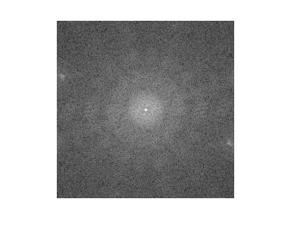
That vertical line in the previous frequency-domain plot is no longer visible.
Since people seem definitely interested in understanding Fourier transforms better, I'll work on putting together more material for the blog. You can help me by continuing to post your comments, including the things that puzzle you.
- Category:
- Fourier transforms


Comments
To leave a comment, please click here to sign in to your MathWorks Account or create a new one.