
Relationship between continuous-time and discrete-time Fourier transforms
Previously in my Fourier transforms series I've talked about the continuous-time Fourier transform and the discrete-time Fourier transform. Today it's time to start talking about the relationship between these two.
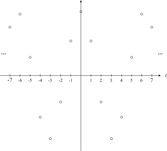
Let's start with the idea of sampling a continuous-time signal, as shown in this graph:

Mathematically, the relationship between the discrete-time signal and the continuous-time signal is given by:

(When I write equations involving both continuous-time and discrete-time quantities, I will sometimes use a subscript "c" to distinguish them.)
The sampling frequency is  (in Hz) or
  (in radians per second).
The discrete-time Fourier transform of  is related to the continuous-time Fourier transform of
  as follows:
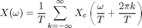
But what does that mean? There are two key pieces to this equation. The first is a scaling relationship between  and
and  :
:  . This means that the sampling frequency in the continuous-time Fourier transform,
  , becomes the frequency
  in the discrete-time Fourier transform. The discrete-time frequency
  corresponds to half the sampling frequency, or
  .
.
The second key piece of the equation is that there are an infinite number of copies of  spaced by .
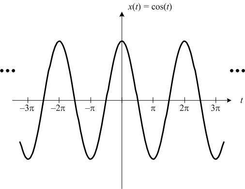
Let's look at a graphical example. Suppose  looks like this:
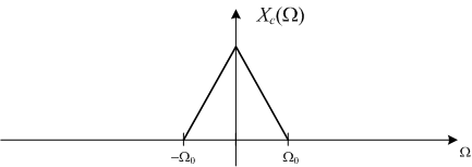
Note that equals zero for all frequencies  . This is what we mean when we say a continuous-time signal is band-limited. The frequency
  is called the bandwidth of the signal.
The discrete-time Fourier transform of looks like this:
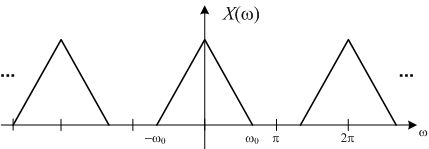
where  . As I mentioned before, normally only one period of
  is shown:
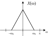
For this example, then, between  and
and  looks just like a scaled version of .
Next time we'll consider what happens when doesn't look like . In other words, we're about to tackle aliasing.
- Category:
- Fourier transforms


Comments
To leave a comment, please click here to sign in to your MathWorks Account or create a new one.