Jähne test pattern – take 2
Last week I talked about the so-called Jähne test pattern and how I found a description of it in Practical Handbook on Image Processing for Scientific Applications, by Bernd Jähne, CRC Press, 1997. This equation was given in the book:

And here's a scan of the test pattern from the book:

I showed how to compute a test pattern based just on sine term. Here's the result:

You can see that the sine-based test pattern extends all the way to the image corners with no decrease in amplitude, whereas the book's test pattern tapers off towards the edges of the image. The book says that "multiplication by the tanh function results in a smooth transition of the ring patterns at the outer edge avoid aliasing problems." That made sense to me, but I couldn't get my generated image to look like what's in the book.
Here's what I tried:
km = pi;
[x,y] = meshgrid(-200:200);
r = hypot(x,y);
rm = max(r(:));
term1 = sin( (km * r.^2) / (2 * rm) );

w = 300;
term2 = 0.5 * tanh((rm - r)/w) + 0.5;
imshow(term2, [])
title('tanh term')
g = term1 .* term2;
imshow(g,[])

That's not much of a taper. I couldn't get my test pattern to look like the figure in the book no matter what value I chose for w. I also noticed that the 2nd term goes down to only 0.5, whereas I would expect a tapering function to range between 0.0 and 1.0. But even when I adjusted the scale and offset of the 2nd term so that it would range between 0.0 and 1.0, I couldn't anything that looked like the book's figure.
So I took a closer look at the shape of  .
.
x = -1:.01:1;
plot(x,tanh(1-abs(x)))

That didn't make sense to me for a taper function. Based on the figure in the book, I expected the taper function to be flatter in the center and to trend more smoothly toward 0 at the edges.
Dear reader, I'm feeling a little dense because I never really figured out this puzzle. If I'm missing something here, please feel free to tell me in the comments. [UPDATE: Reader Alex H. helped me figure out the problem. See this follow-up post.]
I thought about constructing another taper function (maybe the Tukey window?), but I'm not sure how necessary this really is. For example, if you're concerned about aliasing effects because of the high
frequency pattern at the image corners, you could just lower  a bit:
km = 0.5*pi;
g = (sin( (km * r.^2) / (2 * rm) ) + 1)/2;
imshow(g)

I've got one more post planned about this image (fun with bandpass filtering), and then I plan to show you an interesting
way to generate a checkerboard image (chessboard image?) based on the function  .
.


댓글
댓글을 남기려면 링크 를 클릭하여 MathWorks 계정에 로그인하거나 계정을 새로 만드십시오.