Automating the extraction of real data from an image of the data – part 2
I'd like to welcome back my fellow MATLAB Central blogger Brett Shoelson for the second in a three-part series on extracting curve values from a plot. You can find Brett over at the File Exchange Pick of the Week blog, or you can check out his many File Exchange contributions. -Steve
Contents
Quick recap
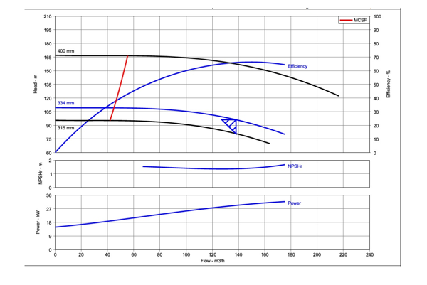
Continuing from last week's guest post, we're heading down the path of extracting real data from the "efficiency curve" in a graphical representation of those data. To recap, here's the original image:
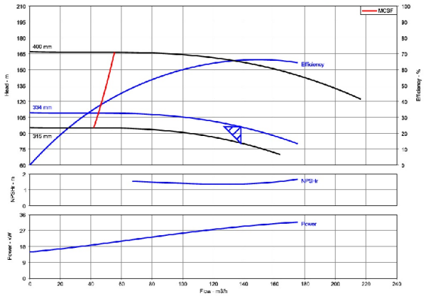
Here are the steps we need to repeat from part 1
url = 'https://blogs.mathworks.com/images/steve/2013/example-pump-perf-curve.jpg';
chart = imread(url);
bw = im2bw(imcomplement(rgb2gray(chart)));
filled = imfill(bw,'holes');
cc = bwconncomp(filled);
stats = regionprops(cc,'Area');
A = [stats.Area];
[~,biggest] = max(A);
filled(labelmatrix(cc)~=biggest) = 0;
bb = regionprops(filled,'BoundingBox'); %We'll use this later!
bb = bb.BoundingBox;
chart(~repmat(filled,[1 1 3])) = 0;
curveOfInterest = rgb2ycbcr(chart);
curveOfInterest = curveOfInterest(:,:,2);
By the end of the first post, I had managed to reduce the SNR so that I ended up with an image (curveOfInterest) that contains a single region...that partially isolates the two blue curves in the top axes:

Next up, segmentation
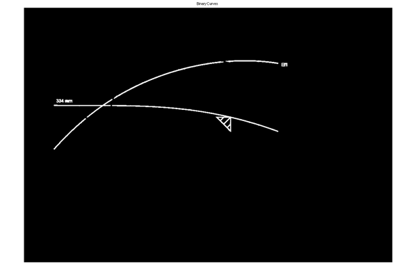
Many (perhaps most) image processing problems require some approach to "segmenting" the image--creating a binary mask that shows white ("true," or 1) where we have signal, and black ("false," or 0) elsewhere. Now that I've masked and converted the original image to YCbCr ("luminance/chrominance/chrominance"), and selected the second (Cb) plane of the resulting image, segmentation is relatively easy. I'm going to use SegmentTool to explore options for doing that:

Simple thresholding works well here (try it!), but I'm going to use a different approach--one that sometimes succeeds where thresholding fails.
curveOfInterest = imextendedmax(im2double(curveOfInterest),0.30,8);
imshow(curveOfInterest)
title('Binary Curves')
Morphologically clean the image
For subsequent analysis, and extraction of data, it will be useful to morphologically alter the image. MorphTool will be your best friend in that regard! ;)

After playing around a bit, I decided to dilate the image, and then to skeletonize it and remove spurs. (bwmorph makes both of those latter processes easy.):
curveOfInterest = imdilate(curveOfInterest, strel('Disk',6));
curveOfInterest = bwmorph(curveOfInterest, 'skeleton', Inf);
curveOfInterest = bwmorph(curveOfInterest, 'spur', 11);
imshow(curveOfInterest)
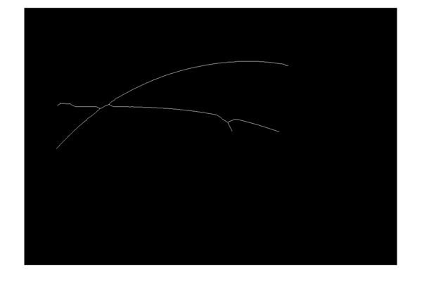
If the curves in that image don't look contiguous, recognize that that's just a screen-resolution issue. There's now exactly one region in this image:
cc = bwconncomp(curveOfInterest);
cc.NumObjects
ans =

     1
Extracting the curve of interest
And now for the difficult part
Okay, we're well on our way. We've eliminated the black and red curves that we don't need, and we've got the curve of interest reduced to a skeleton that contains the minimum information that we do need. But we still have to find a way to extract only the efficiency curve, and to discard the curve representing "334-mm" of head. We can't use color; the curves in the original image are identical. So we're left with differentiating the curves based on their morphological (shape) characteristics.
I'm going to do this two different ways
Sometimes it's useful to be able to trace the boundary of a region, or (as we do here), to trace along a particular path. bwtraceboundary will allow us to do just that.
BWTRACEBOUNDARY
If you've never used it before, take a moment to read the documentation for bwtraceboundary. You'll find that it allows you to operate on a binary image by specifying a starting point (P), an initial trajectory (fstep) along a path in the image, and a direction (dir) in which you want to trace the path. ("Direction" here allows you to specify the overall orientation of the boundary you want to trace.)
Automating the determination of the starting point
Recalling that the curve of interest always starts in the lower left of the upper axes, we can readily automate the determination of the starting point. (It will be the point closest to the bottom left of the masked axes.) I'm going to use regionprops to determine the bounding box of the masked axes (currently contained in variable "filled"). However, the doc for regionprops indicates that BoundingBox is measured from the upper left; I need the lower left so I'll have to manipulate the calculation of the bounding box a bit:
targetPoint = regionprops(filled,'BoundingBox');
targetPoint = targetPoint.BoundingBox(1:2) + [0 targetPoint.BoundingBox(4)];
[ys,xs] = find(curveOfInterest);
Now it remains to get the distance from all points to the lower left corner of the bounding box, and to find the point that minimizes that distance. (I'm going to use a Statistics Toolbox function here, but this is a relatively easy function to write if you don't have that Toolbox.)
[~,ind] = min(pdist2(targetPoint,[xs,ys]));
P = [ys(ind),xs(ind)]; %(Careful here: P is represented as [row,col], not [x,y]!)
Now we need to orient the trace
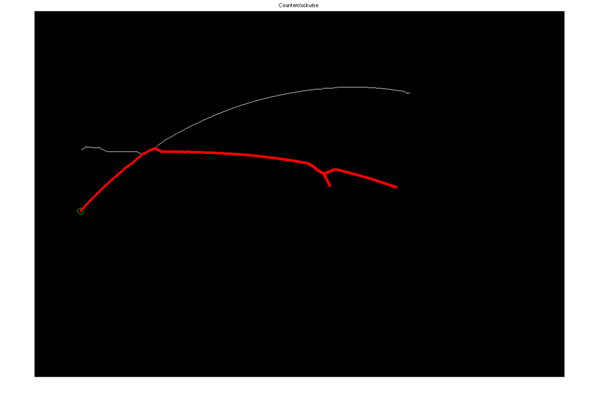
Consider the results using two different orientations:
N = 1000; %If I leave this unbounded (Inf), all points on the curve will be detected!
% Counterclockwise
Bccw = bwtraceboundary(curveOfInterest,P,'NE',8,N,'counterclockwise');
imshow(curveOfInterest);
hold on
plot(P(2),P(1),'go','MarkerSize',12)
plot(Bccw(:,2),Bccw(:,1),'r','LineWidth',5);
title('Counterclockwise')
hold off
Now clockwise.
Bcw = bwtraceboundary(curveOfInterest,P,'NE',8,N,'clockwise');
imshow(curveOfInterest);
hold on
plot(P(2),P(1),'go','MarkerSize',12)
plot(Bcw(:,2),Bcw(:,1),'r','LineWidth',5);
title('Clockwise')
hold off
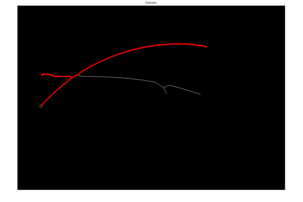
That's interesting; I see that if I specify a clockwise orientation for my curve (and if I use a sufficiently large N), I can constrain the boundary-tracing algorith to roughly follow the efficiency curve I'm after. However, there's a significant spur on the data that may present difficulties when we try to fit the data to a curve that reasonably represents the efficiency-versus-flow rate. If I break this up into smaller pieces and examine the output at each stage, I find that I can significantly improve this result. Here, for instance, I "step" in an easterly direction, initially specifying a counterclockwise orientation. Then I iterate over small chunks, and evaluate the results after each iteration. When the curve stops increasing in the _x-_direction (i.e., when the largest column value isn't equal to the step size), I change the orientation to keep the trace following the desired curve. (Note that there are lots of combinations of parameters that will work here; this step took some experimentation!)
sz = 25;
ind = sz;
nIters = 100;
allBs = nan(sz*nIters,2);
Pnew = P; %reset
h = text(200,385,'Direction:','FontSize',14,...
    'FontWeight','bold','color','w','HorizontalAlignment','left')
for ii = 1:nIters
    if ind == sz
        direction = 'counterclockwise';
    else
        direction = 'clockwise';
    end
    set(h, 'string',['Direction: ',direction])
    %B yields [ROW,COL]:
    B = bwtraceboundary(curveOfInterest,Pnew,'E',8,sz,direction);
    hold on; plot(B(:,2),B(:,1),'r.');drawnow;
    allBs((ii-1)*sz+1:(ii-1)*sz+sz,:) = B;
    [~,ind] = max(B(:,2));
    % Update the starting point, Pnew:
    Pnew = B(ind,:);
end

That result looks great, and will facilitate a good curve fit!
Using regionprops
Anyone who has ever heard me lecture about image processing has likely heard me mention that regionprops can make difficult problems easy. Let's first use bwmorph to find the intersection of the two curves; it will present as a branch point in the skeletonized curve.
branchPoints = bwmorph(curveOfInterest,'branchpoints');
Now dilate that point and use it to break the curves at their branches.
branchPoints = imdilate(branchPoints,strel('disk',3));
curveOfInterest = curveOfInterest & ~branchPoints;
imshow(curveOfInterest)
axis([100 420 180 400])
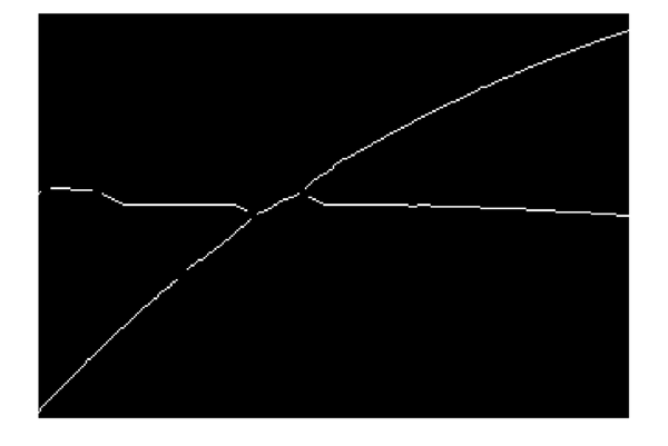
In this zoomed view, we can see that we've now broken the curve into branches. We can also verify that we now have multiple ROIs...
cc = bwconncomp(curveOfInterest)
cc =

    Connectivity: 8
       ImageSize: [738 1067]
      NumObjects: 11
    PixelIdxList: {1x11 cell}
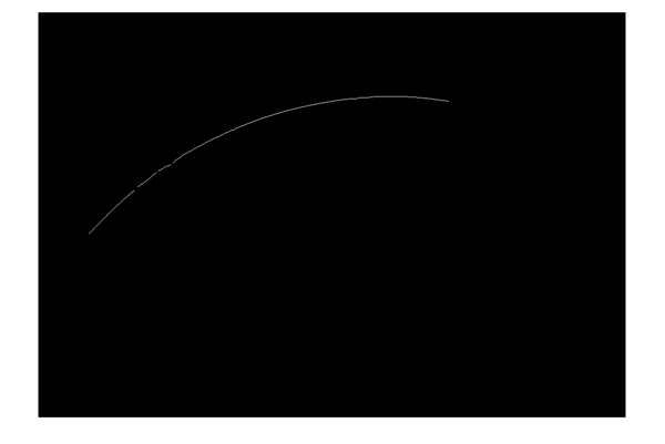
...and we can use their shape properties to select the ones we want. (I will select the ones comprising more than 10 connected pixels, and that have a positive orientation (angle from the horizontal).
stats = regionprops(cc, 'Area','Orientation','Centroid');
idx = find([stats.Area] > 10 & [stats.Orientation] > 0);
curveOfInterest = ismember(labelmatrix(cc),idx);
clf
imshow(curveOfInterest)
figure
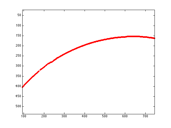
[ys,xs] = find(curveOfInterest);
plot(xs,ys,'r.','MarkerSize',7)
axis ij
axis equal
Next up: fitting a curve
So that essentially wraps up the "image processing aspect" of the problem, and from here, it becomes a problem of fitting a curve. For completeness, I'll hijack Steve's blog one more time to show how the Curve-Fitting Toolbox facilitates that process. See you next week!




评论
要发表评论,请点击 此处 登录到您的 MathWorks 帐户或创建一个新帐户。