 Cleve’s Corner: Cleve Moler on Mathematics and Computing
 The MATLAB Blog
 Guy on Simulink
 MATLAB Community
 Artificial Intelligence
 Developer Zone
 Stuart’s MATLAB Videos
 Behind the Headlines
 File Exchange Pick of the Week
 Hans on IoT
 Student Lounge
 MATLAB ユーザーコミュニティー
 Startups, Accelerators, & Entrepreneurs
 Autonomous Systems
 Quantitative Finance
 MATLAB Graphics and App Building
Timing the FFT
I've seen two questions recently about the speed of the fft function in MATLAB. First, a tech support question was forwarded to development. The user wanted to know how to predict the computation time for an FFT of a given length, N. This user was interested in values of N in the neighborhood of 4096 (2^12).
The second was a post in the MATLAB newsgroup comp.soft-sys.matlab. This user wondered why padding to the next power of two wasn't always the fastest way to compute the FFT.
Inspired by these questions, I want to show you today how to do some FFT benchmarking in MATLAB.
It turns out that, in general, the time required to execute an N-point FFT is proportional to N*log(N). For any particular value of N, though, the execution time can be hard to predict and depends on the number of prime factors of N (very roughly speaking). The variation in time between two close values of N can be as much as an order of magnitude.
Whenever I do FFT benchmarking, I find it very helpful to look at three sets of numbers:
- Powers of 2
- Composite numbers that are not powers of 2
- Prime numbers
Also, I have learned to look at plots that are log scale in N and that have roughly the same number of test values within each octave (or doubling) of N.
Constructing sets of N values along these lines takes a little thought. Here's some code.
First, how many powers of 2 do we want to examine? Based on the customer questions I saw, I want to examine the range from 1024 (2^10) to 131072 (2^17).
low2 = 10;
high2 = 17;
n2 = 2.^(low2:high2);
Next, I want to pick 10 composite numbers and 10 prime numbers in between successive powers of 2. I'd like to pick the numbers "randomly," but I also want my experiment to be repeatable. To satisfy these seemingly contradictory constraints, I'll reset the MATLAB random number generator before beginning.
rng('default');

% Initialize the vectors holding the prime N's and composite N's.
np = [];
nc = [];

for m = low2:high2
    k = (2^m):(2^(m+1));
    kp = k(2:end-1);
    isp = isprime(kp);
    primes = kp(isp);
    composites = kp(~isp);

    % Use randperm to pick out 10 values from the vector of primes and 10
    % values from the vector of composites.
    new_np = primes(randperm(length(primes),10));
    new_nc = composites(randperm(length(composites),10));

    np = [np new_np];
    nc = [nc new_nc];
end
Now let's use the function timeit to measure the execution time required to compute FFTs for all these values of N. (If you don't have a recent version of MATLAB that has timeit, you can get a version of it from the File Exchange.)
t2 = zeros(size(n2));
for k = 1:length(n2)
    x = rand(n2(k),1);
    t2(k) = timeit(@() fft(x));
end
tp = zeros(size(np));
for k = 1:length(np)
    x = rand(np(k),1);
    tp(k) = timeit(@() fft(x));
end
tc = zeros(size(np));
for k = 1:length(nc)
    x = rand(nc(k),1);
    tc(k) = timeit(@() fft(x));
end
Now do a loglog plot of all these times.
loglog(n2,t2,'o')
set(gca,'xtick',2.^(10:17))
xlim([2^10 2^17])

hold on

loglog(nc,tc,'+')
loglog(np,tp,'*')

hold off

legend({'Powers of 2','Composite numbers','Prime numbers'}, ...
    'Location','NorthWest')
xlabel('N')
ylabel('Execution time (s)')
title('FFT execution time as a function of N')
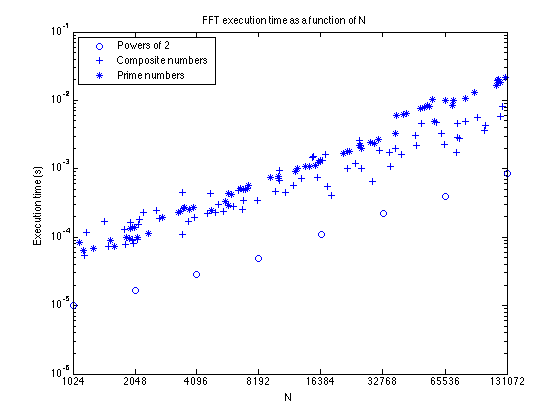
You can see that there's a wide spread of execution times for the values of N that are not powers of 2.
One thing I'm not seeing is what the MATLAB Newsgroup poster reported. That is, I don't see a non-power-of-2 time that's faster than the next highest power of 2.
So let's look a little harder for composite numbers that are faster than what we've seen so far. Specifically, I'm going to look for values of N with prime factors no bigger than 3.
nn = [];
for m = low2:high2
    k = (2^m):(2^(m+1));
    kp = k(2:end-1);

    kp = kp(randperm(length(kp)));
    nn_m = [];
    for q = 1:length(kp)
        if max(factor(kp(q))) <= 3
            nn_m = [nn_m kp(q)];

            if length(nn_m) >= 4
                % We've found enough in this part of the range.
                break
            end
        end
    end

    nn = [nn nn_m];
end
Measure execution times for these "highly composite" numbers.
tn = zeros(length(nn),1);
for k = 1:length(nn)
    x = rand(nn(k),1);
    tn(k) = timeit(@() fft(x));
end
Add the times to the plot.
hold on
loglog(nn,tn,'d')
hold off

legend({'Powers of 2','Composite numbers','Prime numbers', ...
    'Highly composite numbers'},'Location','NorthWest')
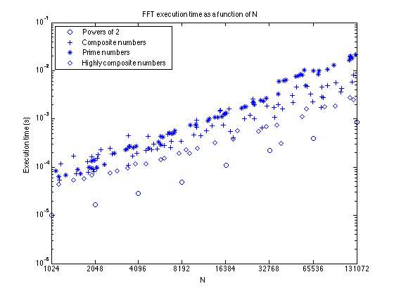
You can see that sometimes a non-power-of-2 can be computed very fast, faster than the next higher power of 2. In this experiment we found one such value of N: 39366. This number has 10 prime factors:
factor(39366)
ans =

     2     3     3     3     3     3     3     3     3     3
I hope you enjoyed these experiments with FFT benchmarking. I can tell you from personal experience that it can turn into almost a full-time hobby!


댓글
댓글을 남기려면 링크 를 클릭하여 MathWorks 계정에 로그인하거나 계정을 새로 만드십시오.