
The curious case of ordfilt2 performance
For today's post, I'd like to welcome guest author Kushagr Gupta, a developer on the Image Processing Toolbox team. -Steve
The Image Processing Toolbox function ordfilt2 can be used to perform various types of 2-D statistical filtering, including minimum or maximum filtering and median filtering. A straightforward implementation of this function is expected to scale with $O(r^2)$, where $r$ is the width of the window (assuming a square window). To compute each output pixel, we have to select the $k$-th largest value from the set of $r^2$ input image pixels, which can be done in $O(r^2)$ time with an algorithm such as quick-select.
The function ordfilt2, however, does better than that; it scales with $O\left(r\right)$complexity. That's because ordfilt2 uses a sliding window-based histogram approach to filter the data. When the algorithm moves from one input image pixel to the next, only part of the histogram needs to be updated. (Reference: Huang, T.S., Yang, G.J., and Yang, G.Y., "A fast two-dimensional median filtering algorithm," IEEE transactions on Acoustics, Speech and Signal Processing, Vol ASSP 27, No. 1, February 1979.)
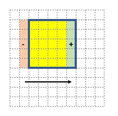
As shown in the figure above, r additions and r subtractions need to be carried out for updating the histogram. Computing the output pixel from the histogram doesn't depend on the window size, and so the overall complexity is $O(r)$.
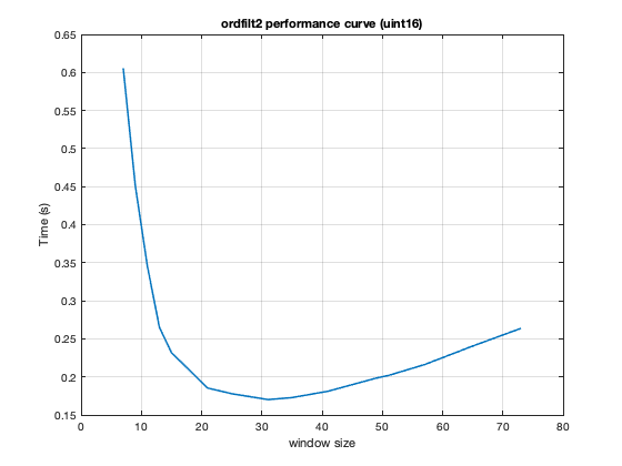
We recently received an interesting tech support case related to performance of ordfilt2 for uint16 random input data. One of our customers reported the time taken to filter an image with a smaller window size was higher than the time taken to process the same image with a relatively larger window size.
Was this just a noisy observation? Was this reproducible? Was this a bug in our implementation?
We investigated?
The customer was generous enough to give us reproduction code. And, the behavior was indeed reproducible! (Many, many times!). What was the explanation?
Here are the reproduction steps:
Im = im2uint16(rand(1e3));
n = [7 9 11 13 15 21 25 31 35 41 49 51 57 65 73];
t = zeros(length(n),1);
for id=1:length(n)
   t(id) = timeit(@() ordfilt2(Im,ceil(n(id)^2*0.5),...
       true(n(id))));
end

plot(n,t)
grid on
title('ordfilt2 performance curve (uint16)')
xlabel('window size')
ylabel('Time (s)')
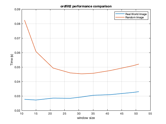
A puzzling aspect of this case was that the performance behavior was observed only for random input data and not for real-world images. Here is a comparison:
Im1 = im2uint16(imresize(imread('coins.png'),[500 500]));
Im2 = im2uint16(rand(500));
n = [11 15 21 27 31 35 41 49 51];
treal = zeros(length(n),1);
trand = zeros(length(n),1);
for id=1:length(n)
   treal(id) = timeit(@() ordfilt2(Im1,ceil(n(id)^2*0.5),...
       true(n(id))));
   trand(id) = timeit(@() ordfilt2(Im2,ceil(n(id)^2*0.5),...
       true(n(id))));
end

plot(n,treal)
grid on
hold on
plot(n,trand)
legend('Real World Image','Random Image')
title('ordfilt2 performance comparison')
xlabel('window size')
ylabel('Time (s)')
hold off
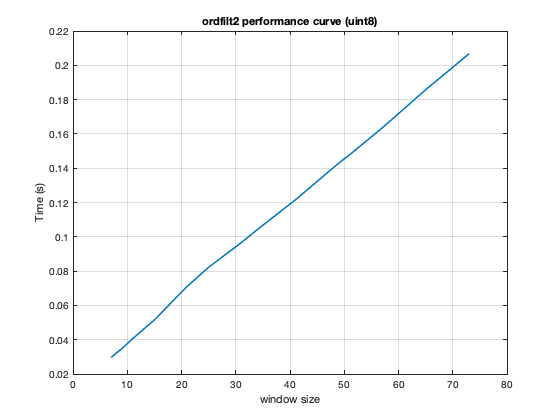
We also observed that the the performance behavior was not reproducible for uint8 random images. Instead, the algorithm's performance scaled linearly with the window size, as expected.
Im = im2uint8(rand(1e3));
n = [7 9 11 13 15 21 25 31 35 41 49 51 57 65 73];
t = zeros(length(n),1);
for id=1:length(n)
   t(id) = timeit(@() ordfilt2(Im,ceil(n(id)^2*0.5),...
       true(n(id))));
end

plot(n,t)
grid on
title('ordfilt2 performance curve (uint8)')
xlabel('window size')
ylabel('Time (s)')
To understand what was going on, it became essential to dig deeper into the inner workings of the underlying algorithm.
As it turns out, while using the sliding window histogram approach, the algorithm also keeps track of the running sum of the histogram so that it does not need to be computed for each pixel in the row. It can be updated accordingly as the window slides by traversing the histogram in the right direction towards the element of interest. This running-sum computation makes the algorithm data dependent. Moreover, the worst case scenario for this data-dependent algorithm happens when the input image contains random data.
But why is the behavior prominently present for small window sizes? It can be argued that, as the window size increases, we draw greater number of samples from the underling distribution resulting in smaller variance. As the variance goes down, the code path becomes more predictable and the algorithm obeys linear time complexity. However, when the window size reduces, the data dependency of the algorithm causes the variance to increase (which is a lot more for random input) making the code path less predictable. This causes the behavior reported by the customer of smaller windows taking more time to process as compared to larger windows.
After some consideration, we have decided to leave the implementation of ordfilt2 as it is. This decision was made based on the fact that the behavior is primarily visible for random input data, which is not usually what customers use ordfilt2 for.


Comments
To leave a comment, please click here to sign in to your MathWorks Account or create a new one.