
How to display images with bilinear interpolation and antialiasing
Note: this blog post describes an image display feature that is new in R2019b. You can download this release from https://www.mathworks.com/downloads.
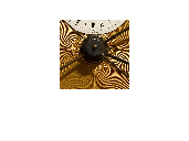
This is my new favorite image:
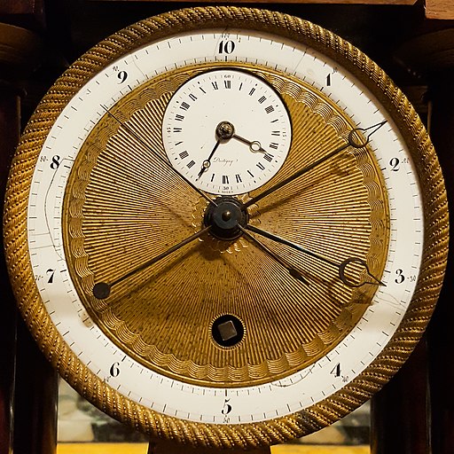
But that's just a 512x512 version of it. Click here for the full resolution (2048x2048) version. Image credit: DeFacto [CC BY-SA 4.0 (https://creativecommons.org/licenses/by-sa/4.0)]
This image caught my eye because I'm always looking for a good sample image to demonstrate aliasing. Also, I wanted to write a blog post about a new MATLAB image display feature in R2019b: bilinear interpolation and antialiasing.
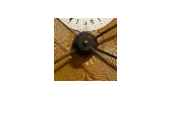
Before I get into image display details, though, let's zoom into the center of the full-resolution image to see why it interests me.
url = 'https://blogs.mathworks.com/steve/files/Decimal_Clock_face_by_Pierre_Daniel_Destigny_1798-1805.jpg';
A = imread(url);
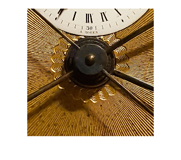
A_cropped = A((-250:250) + 1024, (-250:250) + 1024, :);
imshow(A_cropped)
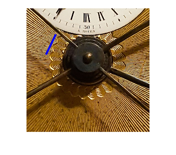
Next, I want to compute a pixel profile along a path that shows the high-frequency spatial variation. The code below shows the path in blue.
hold on
x = [120 80];
y = [106 188];
plot(x,y,'b','LineWidth',4)
hold off
And here's the pixel profile (converted to gray-scale) along that path.
close all
c = improfile(A_cropped,x,y);
c = rgb2gray(squeeze(c)/255);
h = plot(c(:,1));
xlabel('Distance along the profile path')
ylabel('Gray-scale pixel value')
datatip(h,13,0.9614);
datatip(h,25,0.9271);
datatip(h,60,0.9282);
datatip(h,72,0.9133);
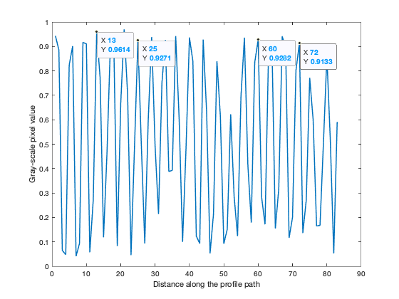
I have placed a few datatips to show that the spatial periodicity along the path is about 4 pixel units. This is very close to the highest spatial frequency that can be represented with this pixel spacing. In other words, it is very close to what I would call critically sampled.
Why does this matter? Well, it means that if you shrink this image down just by using nearest-neighbor interpolation, which is the way MATLAB has always displayed images previously, you'll see some strange artifacts. Below, I'll use imshow to display the image at 25% magnification.
imshow(A_cropped,'InitialMagnification',25)
With R2019b, though, you can specify that you want an image to be displayed using bilinear interpolation. And, as explained in the documentation, when bilinear interpolation is specified, MATLAB also automatically applies an antialiasing technique.
imshow(A_cropped,'InitialMagnification',25,'Interpolation','bilinear')
You can still see some spatial artifacts in this result, but they are significantly reduced.
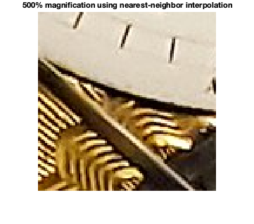
Now let's examine the effect of specifying bilinear interpolation when you magnify an image instead of shrinking it. First, I'll crop out an even smaller piece of the original image.
B_cropped = A_cropped(50:150,115:215,:);
imshow(B_cropped)

Next, let's display it with 500% magnification, with and without the bilinear interpolation option.
imshow(B_cropped,'InitialMagnification',500)
title('500% magnification using nearest-neighbor interpolation')
imshow(B_cropped,'InitialMagnification',500,'Interpolation','bilinear')
title('500% magnification using bilinear interpolation')
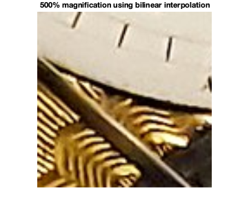
You can see the improved quality in the version using bilinear interpolation.
Note that the default is still nearest-neighbor interpolation. This was a choice that we discussed at some length. Ultimately, we decided to leave the default behavior unchanged, for two reasons:
- to avoid incompatibilities
- for some image arrays, such as those containining segmentation labels or other kinds of categories, bilinear interpolation would not be appropriate
If you already have MATLAB R2019b, give this image display option a try and let me know what you think in the comments.


Comments
To leave a comment, please click here to sign in to your MathWorks Account or create a new one.