
How to Display Color Swatches
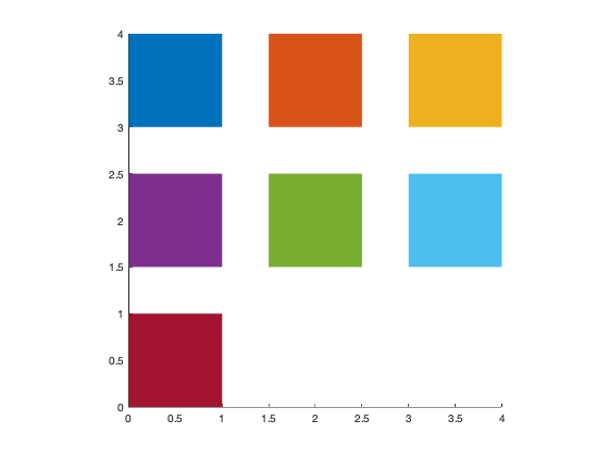
When working on the "Color Image Processing" chapter of DIPUM3E, I found myself often wanting to display square blocks (or swatches) of color, like this:

Eventually, I wrote a function, colorSwatches, to display a bunch of color squares using a single patch object. This function is used in DIPUM3E, and it is included in the MATLAB code files for the book. To call it, start with a set of RGB color values arranged in a Px3 matrix, where P is the number of colors. The lines functions returns the colors used by the MATLAB plot function:
c = lines(7)
c =

         0    0.4470    0.7410
    0.8500    0.3250    0.0980
    0.9290    0.6940    0.1250
    0.4940    0.1840    0.5560
    0.4660    0.6740    0.1880
    0.3010    0.7450    0.9330
    0.6350    0.0780    0.1840
Now just call colorSwatches, passing in the set of colors, and optionally passing in the desired size of the color grid.
grid_size = [3 3];
colorSwatches(c,grid_size)

The color swatches in the above figure are not quite square, and that's because the data aspect ratio in the axes is not 1:1. But we can easily change that using the daspect function.
daspect([1 1 1])
Let's look under the hood and see this all works using just a single patch object.
p = colorSwatches(c,grid_size)
p =

  Patch with properties:

    FaceColor: 'flat'
    FaceAlpha: 1
    EdgeColor: 'none'
    LineStyle: '-'
        Faces: [9×5 double]
     Vertices: [45×2 double]

  Use GET to show all properties

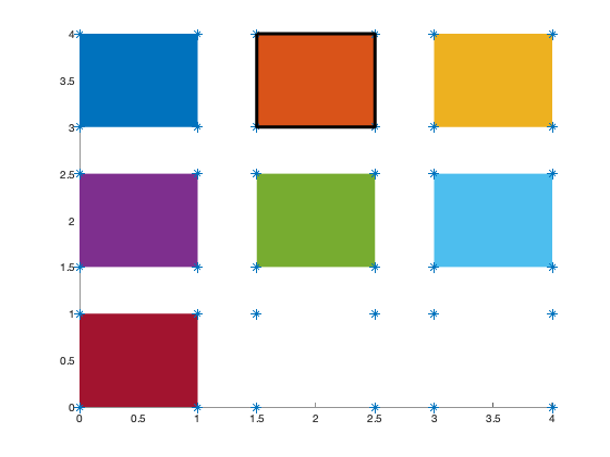
For us, the key properties are Vertices, Faces, and FaceVertexCData. The Vertices property is 45x2, indicating that the patch has 45 vertices. Here they are:
hold on
plot(p.Vertices(:,1),p.Vertices(:,2),'*')
hold off

The Faces property is 9x5, indicating that there are 9 faces, each of which connects 5 vertices. Here is the second row of the Faces property:
face2 = p.Faces(2,:)
face2 =

     6     7     8     9    10
These are indices into the Vertices property. Below, I'll use the Faces and Vertices properties to draw a black line around the second face.
x = p.Vertices(face2,1);
y = p.Vertices(face2,2);
hold on
plot(x,y,'k','LineWidth',3)
hold off
The FaceVertexCData property controls the color of each face. Note that each face has a constant color because the FaceColor property is 'flat'.
p.FaceVertexCData
ans =

         0    0.4470    0.7410
    0.8500    0.3250    0.0980
    0.9290    0.6940    0.1250
    0.4940    0.1840    0.5560
    0.4660    0.6740    0.1880
    0.3010    0.7450    0.9330
    0.6350    0.0780    0.1840
       NaN       NaN       NaN
       NaN       NaN       NaN
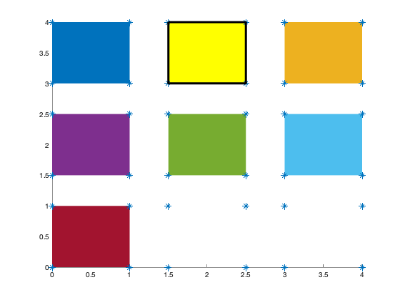
If we change the numbers on the second row of the FaceVertexCData property, then the color of the second face will change.
p.FaceVertexCData(2,:) = [1 1 0];
Another application of colorSwatches is to draw a color ramp. For example, we can visualize the parula colormap by using a single row of color swatches, setting the gap between each swatch to 0, and controlling the data aspect ratio to make it look like a long, thin bar.
parula_colors = parula(256);
gap = 0;
colorSwatches(parula_colors,gap,[1 256])
daspect([30 1 1])
axis off

One final note: when I wrote colorSwatches, I didn't want it to have any side effects on the axes properties, and that's why I didn't write it to automatically set the axes DataAspectRatio. I do think, though, that having color swatches that are actually square is sufficiently common to write a function for it, so I have added squareColorSwatches to MATLAB Color Tools. Here it is in action:
squareColorSwatches(c,[3 3])


Comments
To leave a comment, please click here to sign in to your MathWorks Account or create a new one.