
Making Color Spectrum Plots – Part 1
The new edition of Digital Image Processing Using MATLAB (DIPUM3E) contains a number of MATLAB functions related to color, color calculations, and color visualization. I wrote about functions for displaying color swatches in my March 10 post. You can find some of the functions in MATLAB Color Tools on the File Exchange, as well as in the GitHub repository containing the MATLAB source code for the book.
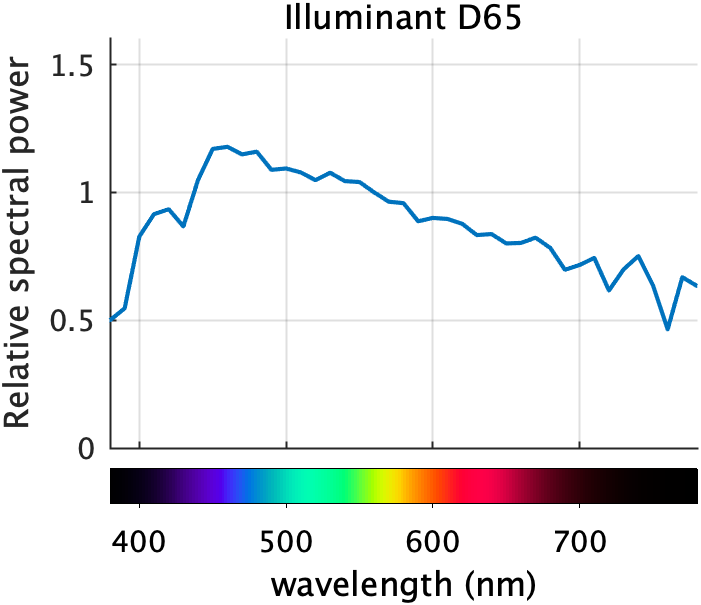
A MathWorks friend asked me, earlier this year, why I chose to write the specific color-related functions that I did. The answer is that I wrote the functions that would help tell the story I wanted to tell. For example, I wanted to talk early in the chapter about the interactions between illumination, object reflectance, and the color sensitivity of retinal receptors in the eye. To help with that story, I wanted to include plots like DIPUM3E Figure 7.2(a):
I thought I would give you a tour of the various algorithms and functions that went into making this and similar plots, including:
- MATLAB functions readtable, interp1, conv2, linspace, colorbar
- Image Processing Toolbox functions xyz2rgb, lin2rgb
- DIPUM3E functions illuminant, lambda2xyz, colorMatchingFunctions, spectrumColors, spectrumBar
I expect the tour to take a couple more blog posts.
First, where does the data in the plot come from? The curve is called a relative spectral power distribution curve. This particular curve is for a standard illuminant called D65, which is intended to approximate average mid-day daylight. The curve is a reference curve created by the International Commission on Illumination, usually written as CIE for the French acronym.
I could have provided this standard data in a MAT-file, I suppose, but I chose instead to provide it as a spreadsheet file, Illuminants.xlsx. Here's what it looks like:
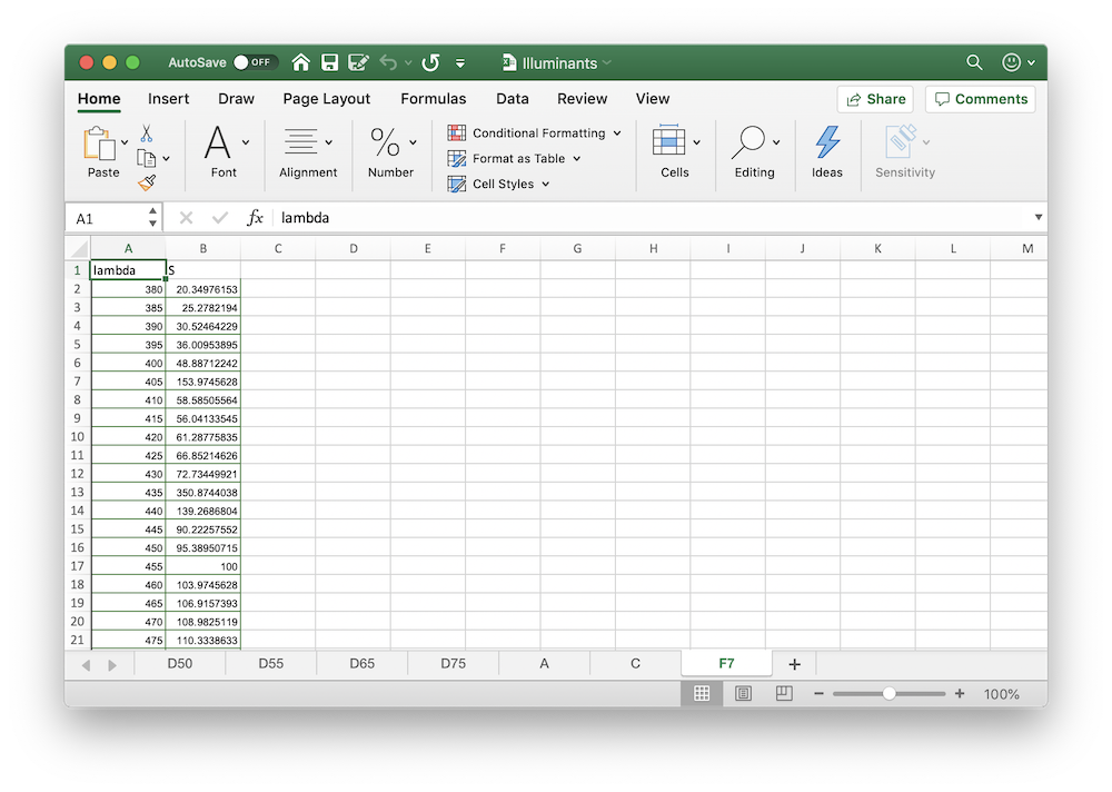
Along the bottom, you can see that the file contains several sheets: D50, D55, D65, D75, A, C, and F7. These sheets contain the data for different types of illuminants.
My tool of choice for reading an Excel file like this is readtable. In the call below, I indicate that I don't want readtable to invoke Excel (this is now the default behavior), and I also indicate that I want to read the D65 sheet.
T = readtable('Illuminants.xlsx','UseExcel',false,'Sheet','D65');
The DIPUM3E function illuminant is basically just this call to readtable.
And here's what the resulting MATLAB table looks like:
head(T)
ans =

  8×2 table

    lambda      S
    ______    ______

     300      0.0341
     305      1.6643
     310      3.2945
     315      11.765
     320      20.236
     325      28.645
     330      37.053
     335      38.501
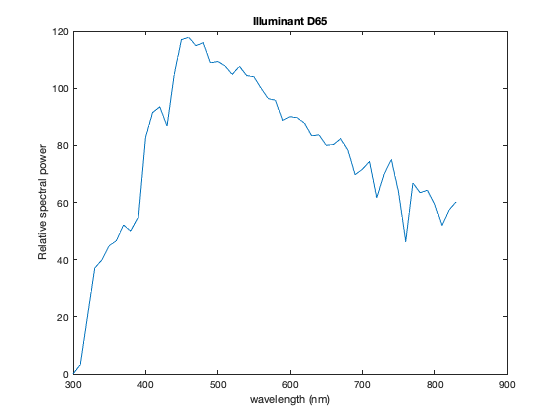
I can produce a basic plot like this:
plot(T.lambda,T.S)
xlabel('wavelength (nm)')
ylabel('Relative spectral power')
title('Illuminant D65')
Next time, I'll talk about computing the rainbow colors that appear at the bottom of DIPUM3E Figure 7.2(a):


Comments
To leave a comment, please click here to sign in to your MathWorks Account or create a new one.