In today’s post, Wojciech Regulski introduces you to modeling fluid dynamics using MATLAB. Wojciech has a PhD in mechanical engineering from Warsaw University of Technology, Poland, and has specialized in Computational Fluid Dynamics (CFD) in his research work. Wojciech also co-founded the QuickerSim company that specializes in development of  fluid flow simulation software.

–  –

Introduction

CFD modeling has become indispensable in many areas. It is used to determine flow conditions such as velocity, pressure, or temperature for diverse kind of problems. Knowing these is pivotal for e.g. automotive or aircraft aerodynamics, heating or cooling problems and even weather forecasts or climatology.

Depending on the extent and complexity of its application, CFD requires:

1. lots of computing resources,
2. dedicated software and
3. quite sophisticated engineering knowledge.

As you are reading this post, let’s not worry too much about #3. #1 becomes more and more negligible as even laptops come with multi-core CPUs and even GPUs. #2 will be tackled in this post; we want to give you an idea of a basic CFD simulation in MATLAB. We will also share example and give insights into projects that student teams are currently conducting.

CFD Modeling in MATLAB

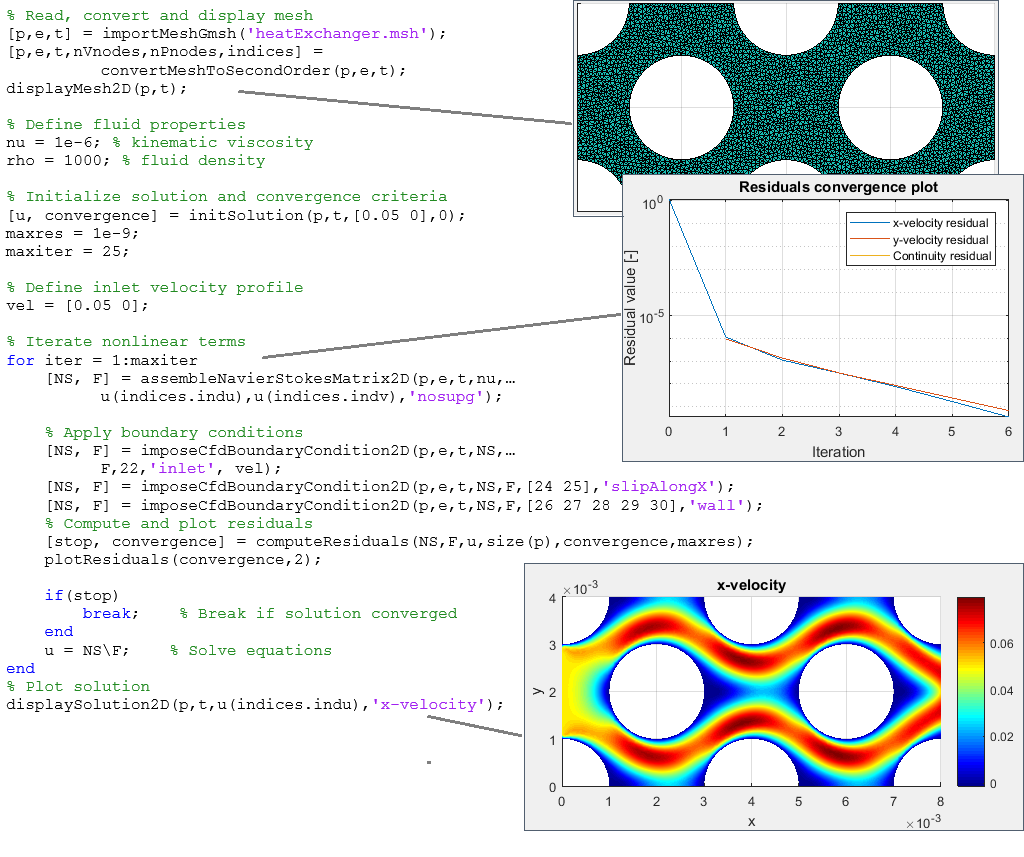
QuickerSim CFD Toolbox, a dedicated CFD Toolbox for MATLAB, offers functions for performing standard flow simulations and associated heat transfer in fluids and solids. The toolbox is based on the Finite Element Method (FEM) and uses the MATLAB Partial Differential Equation Toolbox™ data format. It operates much like a standard CFD solver – a set of routines executes consecutive simulation steps, see Figure 1. First, the computational mesh is read in and the solution is initialized. Then the iterative process of solving the equations takes place. Finally, the user can resort to various post-processing tools and manipulate the data flow on his own.

Fig. 1. Script and illustration of a flow simulation past an array of pipes.

CFD Best Practices for Student Competition Teams

While practically any aspect of a car design is subject to CFD analysis, many areas are very demanding. Topics such as fuel combustion or noise generation are tackled only by large and experienced engineering departments. Also, the numerical models used there are very complex and have been validated using extensive experimental trials. Still, areas such as battery cooling or simple aerodynamic cases can be analyzed using standard tools by individuals in relatively short time frames.

Simulating of Heating and Cooling

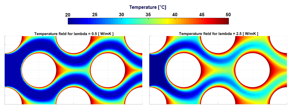
Figure 2 shows results of a 2-Dimensional heat exchanger simulation where the fluid passes past an array of pipes perpendicular to the flow direction as already shown in Figure 1. Observe the development of the so-called thermal boundary layer on the pipe walls, whose thickness depends on the fluid properties. Resolving flow and heat phenomena in the vicinity of the solid walls is critical for accurate prediction of heat fluxes and aerodynamic drag. The toolbox contains a set of functions that lets you generate and improve the boundary layer mesh.

Although the geometry here is simple, the basic rule remains the same for more complex cases. First, one resolves the fluid flow, what constitutes most of the computational effort. On top of that, the heat transfer equations are solved, which is less expensive computationally. All that is performed by 40 lines of code within a few minutes of calculation on a laptop.

You can get the code here: https://quickersim.com/cfdtoolbox/tutorial/tutorial-15-laminar-heat-exchanger/

Fig. 2. A 2D simulation of a laminar heat exchanger. Temperature fields for two different thermal conductivities

Cooling of a Battery Pack

The SAE team Form UL from Université Laval, Québec, has created a numerical model of their racing car in MATLAB. One of its modules deals with the issue of unsteady heat transfer in the batteries shown in Figure 3. Pierre Olivier Cimon, one of the team leaders and the developer of this model, recognizes its limitations. “Standard engineering correlations do not account for the transient effects and the flow confinement in the compartment. Hence, we resorted to the QuickerSim CFD Toolbox with hope of getting better heat transfer and pressure drop data.”

Fig. 3 The battery pack as used by the Form UL SAE Team from Canada

The work is still in progress, since the team would like to simulate the entire 30-minute-long run of the car. This can hardly be achieved with a direct simulation and rather requires a clever choice of simplifying assumptions.

The first step is the evaluation of the numerical model for the unsteady flow with conjugate heat transfer using just a few battery cells. You can check out the joint movie below for the initial results.

Car Aerodynamics

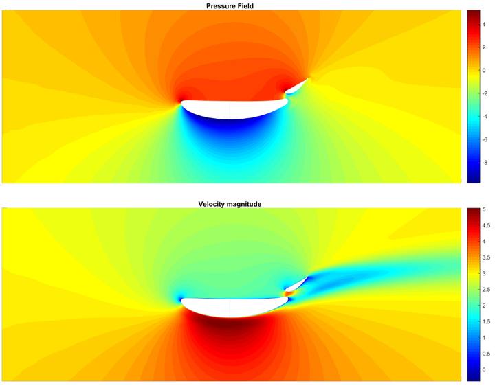
Team Strom + Söhne from TH Nürnberg, employed the toolbox in their design of the spoiler, see Figure 4. “We aim to increase the downward force of our vehicle while keeping the drag as low as possible”, says Andreas Fischer, one of the leaders of Strohm + Söhne. Simulating the entire component is a Formula 1-level of complexity challenge, but one can still get valuable insights using 2D simulations. The first results for their aileron-flap system are shown in Figure 5 below. You can notice the under-pressure zone on the lower side of the airfoil.

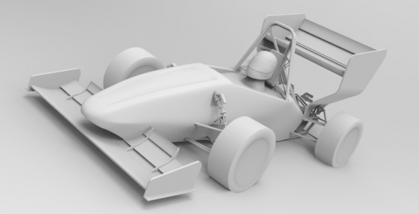
Figure 4. The perspective view of the racing car of Strohm + Söhne team.

The most challenging simulations will be those where the flap is significantly deflected. The flow will most likely become very chaotic and steady CFD-models will be of little use then. Before that, however, the steady-state turbulence models (the so-called RANS models) give accurate results.

Fig. 5 The velocity and pressure fields around the spoiler of the S+S Team form Nürnberg.

Automated Airfoil Optimization

Indeed, one will often look for improvement of the airfoil performance by manipulating its shape. Usually he would like to maximize the lift-to-drag ratio (L/D). Such a procedure can be carried out automatically. A basic turbulent flow simulation from the toolbox is hence nested in the MATLAB optimization code. In each optimization step the mesh is deformed accordingly and another CFD simulation is carried out.

Below you can check out the movie showing the outcomes of consecutive steps of such procedure. Watch the large initial variations of the trailing edge shape and the ratio L/D. After just a few steps the improvements are only slight and the process is terminated.

You can get the code here: https://quickersim.com/cfdtoolbox/tutorial/tutorial-22-automatic-shape-optimization/

Conclusion

To sum up, we hope that we managed to convince you that:

1. Basic flow cases can be dealt with in MATLAB as part of a larger workflow.
2. Even complex 3D flow problems can be approximated with 2D surrogates.

If you want to test the QuickerSim CFD Toolbox yourself, is available here: https://quickersim.com/cfdtoolbox/download/. The basic version is free of charge, it deals with steady laminar flows and heat transfer in two dimensions only. If you want to unlock the full potential, just ask us for the trial license. The teams belonging to the Racing Lounge may get a free access the full license for the whole year – just contact us at contact@quickersim.com