
Deep Chimpact: Depth Estimation for Wildlife Conservation – MATLAB Benchmark Code
As promised in our last blog, here we are with the MATLAB benchmark code for the Deep Chimpact: Depth Estimation for Wildlife Conservation Challenge.
James Drummond, from MathWorks Engineering Development group, took a stab at this challenge and prepared this starter code. Here he will talk about the optical Flow + CNN aproach he used for solving the problem. He will also throw some tips and tricks in between on how you can improve this code and improve your score.
Checkout the links below to sign up for the challenge, receive your complimentary MATLAB Licenses, and visit the discussion forum for support.

The Data
The objective of this challenge is to estimate the distance to animals in monocular trail camera footage. The videos are in both color and grayscale for night vision and contain a range of different animals as subjects.
The dataset consists of over 3,500 videos (nearly 200GB of data) split into a training and a test set. These are hosted in a public S3 bucket. Instructions for accessing this can be found on the competition Data tab.
Each video is given a unique 4 letter name and is either .mp4 or .avi format. The labels are provided (“train_labels.csv” & “test_labels.csv”) as the distance to the center of gravity of the animal at specific timestamps in each video. To help facilitate faster data processing a down-sampled version of each file is also provided.
In addition, you are provided with “train_metadata.csv” and “test_metadata.csv” files. These files consist of information like filename, details about where the camera was located, and a model-generated estimate of the bounding box for the animal at each timestamp.
For further details about the dataset check out the Problem Description on the competition webpage.
Getting Started with MATLAB
I am providing a basic example code in MATLAB to serve as a starting point for development. In this code, I use optical flow to pre-process the video frames and feed these images into a basic regression model, using a pre-trained CNN. Then, I will use this model to conduct depth estimation on test data and save a CSV file in the format required for the challenge. You can also download this MATLAB starter code from this GitHub repo. This can serve as basic code where you can start analyzing the data and work towards developing a more efficient, optimized, and accurate model. Additionally, I have provided a few tips and suggestions for next steps to investigate.
So, let’s get started with this challenge!
Load labels and metadata
The first step is to load the information about the dataset you will be using. To access the variable values from the files train_metadata.csv and train_labels.csv, I import them into MATLAB using the readtable function:
labels = readtable('train_labels.csv');
head(labels)

metadata = readtable('train_metadata.csv');
head(metadata)
 Access & Process Video Files
Datastores in MATLAB are a convenient way of working with and representing collections of data that are too large to fit in memory at one time. It is an object for reading a single file or a collection of files or data. The datastore acts as a repository for data that has the same structure and formatting. To learn more about different datastores, check out the documents below:
- Getting Started with Datastore
- Select Datastore for File Format of Application
- Datastores for Deep Learning
In this blog, I will be using an imageDatastore to load the videos from the S3 bucket. Each video is processed using the readVideo helper function outlined in the section below. I save the datastore in a MAT-file in tempdir or current folder before proceeding to the next sections. If the MAT file already exists, then load the datastore from the MAT-file without reassessing them.
Here, I am using the down sampled videos to save bandwidth and processing time. Each video is reduced to a single frame per second which is sufficient for my needs. To access the full videos, you will need to replace the URL of the file on S3 bucket.
tempimds = fullfile(tempdir,"imds.mat");
if exist(tempimds,'file')
    load(tempimds,'imds')
else
    imds = imageDatastore('s3://drivendata-competition-depth-estimation-public/train_videos_downsampled/',...
                          'ReadFcn',@(filename)readVideo(filename,metadata,'TrainingData'),...
                          'FileExtensions',{'.mp4','.avi'});
    save(tempimds,"imds");
end

files = imds.Files;
Tip: (Optional) In order to reduce processing times, you can choose to use a subset of the imageDatastore for your initial investigations:
rng(0); %Seed the random number generator for repeatability
idx = randperm(numel(files));
imds = imds.subset(idx(1:100)); %Random Subset for testing
Extracting video frames & Optical Flow
Once I have the imageDatastore, I extract the video frames by defining a custom read function readVideo (code at the end of this file), which starts by loading the desired video using a VideoReader object. As the downsampled videos have a single frame per second, the videos can simply be indexed to extract the necessary frames.
Optical Flow
Optical flow is the distribution of the apparent velocities of objects in an image. By estimating optical flow between video frames, you can measure the velocities of objects in the video.
For each labeled frame, I calculate the optical flow compared to the previous frame/second. If we assume that the animals are moving against a mostly stationary background, the optical flow highlights where they are and provides some context as to their movement. To improve the signal-to-noise ratio, the provided bounding box estimate is used to generate a binary mask for the region of interest. This is used in place of simply cropping the images to retain any spatial context.
More information on the techniques used can be found at the following links:
To help with processing later on,each image is named with the video it comes from and the timestamp. Here is an example output for Frame 0 of video aany.mp4:

This clearly shows the monkey position and size relative to the rest of the image but the mask avoids background noise.
In order to generate the complete dataset, I read all of the videos using the following command. Here, I use the Parallel Computing Toolbox to speed up the processing as each video can be read independently.
imds.readall("UseParallel", true);
Designing the Neural Network
In this example, I am going to perform transfer learning using a pre-trained network, ResNet-18. However, before you can progress to the actual learning, the network needs to be adapted to match our needs. In particular, the input and output layers need to be replaced. ResNet-18 takes 224x224x3 input images and outputs an image classification with 1000 categories. Whereas, I will be inputting 480×640 images and outputting a single regressed distance estimate.
In MATLAB these changes can be achieved in two ways, either programmatically or graphically using the Deep Network Designer app.
Both approaches start by installing the Deep Learning Toolbox Model for ResNet-18 Network from the Add-on Explorer.

Approach 1: Using Deep Network Designer
This application can be found in the Apps ribbon or by running the command:
deepNetworkDesigner
From the start-up page, import the pre-trained ResNet-18 network:

On the input side, I replace the 224x224x3 imageInputLayer with my own 480×640 imageInputLayer. In order to connect to the rest of the network, the image will then need to be resized to 3D using a resize3dLayer layer with ‘OutputSize’ 480x640x3.

Next on the output side, I remove the last few layers and replace them with my own. In particular, I replace the fullyConnectedLayer, the softmaxLayer and the classificationLayer with a final fullyConnectedLayer to give only a single output value – the distance estimate – which will feed into an output regressionLayer.

After making these changes, you can export this network to your workspace to use in training. The network is exported as a LayerGraph called ‘lgraph_1’.
Approach 2: Create network programmatically
Alternatively, you can apply these changes programmatically. After installing the ResNet-18 Add-on, you can import the trained network.
lgraph_1 = layerGraph(resnet18);
On the input side, I replace the 224x224x3 imageInputLayer – named ‘data’ – with my own 480×640 imageInputLayer. In order to connect to the rest of the network, I resized the image to 3D using a resize3dLayer layer with ‘OutputSize’ 480x640x3.
inputLayers = [imageInputLayer([480 640],'Name','imageinput'),...
              resize3dLayer('OutputSize',[480 640 3],'Name','resize3D-output-size')]

lgraph_1 = replaceLayer(lgraph_1,'data',inputLayers);
Next on the output side, I remove the last few layers and replace them with my own. In particular, the fullyConnectedLayer ‘fc1000’, softmaxLayer ‘prob’ and classificationLayer ‘ClassificationLayer_predictions’ with the final fullyConnectedLayer to give only a single output value – the distance estimate – which will feed into an output regressionLayer.
lgraph_1 = removeLayers(lgraph_1,{'fc1000','prob','ClassificationLayer_predictions'})
outputLayers = [fullyConnectedLayer(1,'Name','fc'),regressionLayer('Name','regressionoutput')]

Now I add the output layers to the end of the layer graph. I then connect the ‘pool5’ and ‘fc’ with the layer graph.
lgraph_1 = addLayers(lgraph_1,outputLayers);
lgraph_1 = connectLayers(lgraph_1,'pool5','fc');
More information about Layer Graphs and the object functions used above can be found here: layerGraph
Analyze network
You can then run the Network Analyzer to confirm that our new layers fit correctly. The results should show a 480×640 input being rescaled to 480x640x3, running through the pre-trained network and then being output as a single regression value.
analyzeNetwork(lgraph_1)


Prepare Training Data
Now that I have completed our pre-processing and have designed the network, the next step is to prepare the data for training.
First, I create our dataset. This consists of a CombinedDatastore, made up of an imageDatastore for the input images and an arrayDatastore for their labels. The generateLabelDS helper function is necessary to ensure the images and labels match up correctly. Reading from the combinedDatastore, ‘fullDataset‘, returns the image and corresponding label.
imageDS = imageDatastore('TrainingData');
labelDS = generateLabelDS(imageDS,labels);
fullDataset = combine(imageDS, labelDS);
Here, I prepare the data for training by partitioning the data into training and validation partitions. I assign 80% of the data to the training partition and 20% to the validation partition.
n_images = numel(imageDS.Files);
n_training = round(0.8*n_images);
idx = randperm(n_images);

trainingIdx = idx(1:n_training);
validationIdx = idx(n_training+1:end);

trainingDS = subset(fullDataset,trainingIdx);
validationDS = subset(fullDataset,validationIdx);
Specify Training Options
As the next step, I specify the training options using the trainingOptions function:
- Set a mini-batch size 8.
- Set an initial learning rate of 0.01.
- Shuffle the data every epoch.
- Validate the network once per epoch.
- Display the training progress in a plot and suppress verbose output.
miniBatchSize = 8;
validationFrequency = floor(n_training/miniBatchSize);

options = trainingOptions('sgdm', ...
    'MiniBatchSize',miniBatchSize, ...
    'MaxEpochs',50, ...
    'InitialLearnRate',0.01, ...
    'Shuffle','every-epoch', ...
    'ValidationData',validationDS, ...
    'ValidationFrequency',validationFrequency, ...
    'Plots','training-progress', ...
    'Verbose',true, ...
    'ExecutionEnvironment',"auto");
Train the Network
I now train the network using the trainNetwork function and save the output to file. Note that this function can take a long time to run, depnding on the type of computaion (GPU, CPU) used.
[net,info] = trainNetwork(trainingDS,lgraph_1,options);
save('trainedNetwork.mat',net)

Using a single Titan Xp GPU, training on the full dataset for 50 epochs took nearly 5 hours. However, this training could have been ended earlier given the performance plateaued in the latter half. Equally, initial investigations were conducted on a subset of the data and so training was much quicker.
Prepare Test Data
Just as I did with the training data, I will now read the test files in an imageDatastore and extract the optical flow of the necessary frames.
test_metadata = readtable('test_metadata.csv');
imds = imageDatastore('s3://drivendata-competition-depth-estimation-public/test_videos_downsampled/',...
                      'ReadFcn',@(filename)readVideo(filename,test_metadata,'TestData'),...
                      'FileExtensions',{'.mp4','.avi'});

imds.readall("UseParallel",true);
Depth Estimation Using Test Data
Using the above trained network, I now perform predictions on the test set. To do so, I use the predict method of the trained network. The predict method takes in a 480×640 image and returns the depth estimation. By looping over all images in the test set I produce a table of results. Here, I am creating a 11933 (the number of test frames) row table with columns: video_id, time and distance.
% Initialise output table

results = table('Size',[height(test_metadata) 3],'VariableTypes',{'string','string','single'},...
          'VariableNames',{'video_id','time','distance'});

for i = 1:height(test_metadata)
    id = test_metadata.video_id{i};
    t = test_metadata.time(i);
    filename = [id(1:4) num2str(t) '.png']; %Find corresponding image name
    file = fullfile('TestData',filename);
    if isfile(file) %Frames without bounding boxes will not have input images
        I = imread(file);
        prediction = predict(net,I,'ExecutionEnvironment','auto');
    else
        prediction = 0;
    end

    results.video_id(i) = id;
    results.time(i) = t;
    results.distance(i) = prediction;
end
head(results)

Save Submission to File
The table of results produced above matches the desired format for submissions so all you need to do now is to save it to a CSV file. This is the file you will submit for the challenge.
writetable(results,'Submission.csv');
Helper Functions
Video pre-processing – Optical Flow
This helper function extracts and pre-processes the labeled frames in the down sampled videos. It then saves these to the supplied folder – ‘/TrainingData‘ in this example.
This is where we are calculating the optical flow of the necessary frames and then using the bounding box to apply a binary mask.
function output = readVideo(filename, metadata, folder)
    %Load video
    vr = VideoReader(filename);
    H = vr.Height;
    W = vr.Width;

    [~, name] = fileparts(filename);
    idx = contains(metadata.video_id,name);

    videoMetadata = rmmissing(metadata(idx,:));   %Ignore frames without bounding box
    n_Frames = height(videoMetadata);

    %Preallocate the output image array
    output = zeros(480,640,n_Frames);

    for i = 1:n_Frames
        opticFlow = opticalFlowLK('NoiseThreshold',0.009);  %Define optical flow
        t = videoMetadata.time(i);  %Extract timestamp
        try
            if t == 0               %If first frame compare with second
                f1 = vr.read(1);
                f2 = vr.read(2);
            else                    %Otherwise take current frame (t+1) and previous (t)
                f1 = vr.read(t);
                f2 = vr.read(t+1);
            end
        catch
            continue %Ignore videos where timings do not match with frames
        end

        %Convert to grayscale
        f1Gray = im2gray(f1);
        f2Gray = im2gray(f2);

        %Calculate optical flow
        estimateFlow(opticFlow,f1Gray);
        flow = estimateFlow(opticFlow,f2Gray);

        %Extract corners of bounding box
        x1 = videoMetadata.x1(i);
        x2 = videoMetadata.x2(i);
        y1 = videoMetadata.y1(i);
        y2 = videoMetadata.y2(i);

        %Apply mask for bounding box
        mask = poly2mask([x1 x2 x2 x1]*W,[y1 y1 y2 y2]*H,H,W);
        maskedFlow = bsxfun(@times, flow.Magnitude, cast(mask, 'like', flow.Magnitude));
        maskedFlow = imresize(maskedFlow,'OutputSize',[480 640]);

        file = fullfile(folder, [name num2str(t) '.png']); %Generate file name

        %Save image to file
        if isfolder(folder)
            imwrite(maskedFlow,file)
        else
            mkdir(folder)
            imwrite(maskedFlow,file)
        end
        output(:,:,i) = maskedFlow;
    end
end
Create arrayDatastore for responses
This function takes in a datastore of images and a table of labels. It then builds an arrayDatastore of labels ensuring correspondence with the image files.
function labelDS = generateLabelDS(imds,labels)
    files = imds.Files;
    n_files = length(files);
    dataLabels = zeros(n_files,1);
    for i = 1:n_files
        [~,id] = fileparts(files{i});
        video = id(1:4);
        time = str2double(id(5:end));
        idx = (contains(labels.video_id,video)) & (labels.time == time);
        dataLabels(i) = labels.distance(idx);
    end
    labelDS = arrayDatastore(dataLabels);
end
Next steps for improvement
Throughout this example there are a number of design choices that I investigated and can be used for improving the score:
Optical Flow
- Algorithm – MATLAB offers 4 techniques for calculating the optical flow. I chose Lucas-Kanade method based on the visual appearance.
- Parameters – The noise threshold is a trade-off between signal and background noise.
- Region of Interest – I have chosen to apply a binary mask to highlight the region of interest but there may be a better approach. Additionally, in this example I have ignored frames without a bounding box. Instead, you could try including the whole optical flow image.
Training data partitioning
- Proportion – changing the proportions of your training and validation data can help control performance and overfitting.
- Method – In this example, the images are split randomly. However, you could also split based on videos or camera site. Please note, that the test data is taking from different sites than those in the training set.
Transfer Learning
- Transfer learning – Here I start with a pretrained neural network and perform additional training based on the competition data – a process called transfer learning. Here we allow all layers of the pretrained model to change during the retraining process (all weights are unfrozen). However, this means we may be losing some of the model’s existing knowledge. Instead, the first step of transfer learning is usually to train only the final layer of a pretrained model on new data, keeping all earlier layers unchanged. Once the new layer is trained, earlier layers can be better fine-tuned without losing insight from the model’s pretraining. This can also be performed by freezing weights of initial earlier layers.
- Freeze Weights – By setting the learning rates of the initial layers to 0, we can prevent the weights from being updated by subsequent learning. More information can be found here.
- Pre-trained network – MATLAB provides numerous options for pretrained networks for you to investigate.
- Training options – Adapting the parameters for training can have a significant on the final results. For example: learning rate, mini batch size, momentum, gradient threshold, loss function
This code can be downloaded from this GitHub Repo. We provide this code as a starting point and are excited to see what innovations you can come up with. Good luck!
- Category:
- Data Science


Comments
To leave a comment, please click here to sign in to your MathWorks Account or create a new one.