What is a Surface?

What is a Surface?

What exactly is MATLAB doing when we say the following?

surf(peaks)

The answer seems obvious. We're telling MATLAB to draw a continuous surface through the points which are defined in the array which the function peaks returns. But where does that surface go in between those points? It turns out that there are some subtle issues hiding here, so let's look a bit closer.

We'll start with a smaller array so that we can see what's really going on.

rng(0)
z = randn(5,7)

z =

    0.5377   -1.3077   -1.3499   -0.2050    0.6715    1.0347    0.8884
    1.8339   -0.4336    3.0349   -0.1241   -1.2075    0.7269   -1.1471
   -2.2588    0.3426    0.7254    1.4897    0.7172   -0.3034   -1.0689
    0.8622    3.5784   -0.0631    1.4090    1.6302    0.2939   -0.8095
    0.3188    2.7694    0.7147    1.4172    0.4889   -0.7873   -2.9443

Let's give that to surf and see what it draws.

f1 = figure;
h = surf(z);
h.FaceColor = 'interp';
h.Marker = 's';
h.MarkerFaceColor = [.7 .2 .3];
h.MarkerEdgeColor = 'none';
title('surf')

Those little grey squares are the values in the array z. It looks like the surface is interpolating linearly between those values. Is that actually what's happening? And is it the best choice?

MATLAB has a useful function named interp2 which will interpolate between the values in a 2D array. We can use interp2 to do the same sort of interpolation that surf is doing, but with more control over the interpolation.

First we'll create a high-res version of the X & Y coordinates of that surface. I've just increased the resolution by a factor of 10, but you could use any number.

[n, m] = size(z);
[x, y] = meshgrid(1:m,1:n);         % low-res grid
[x2,y2] = meshgrid(1:.1:m,1:.1:n);  % high-res grid

Then we'll use interp2 to interpolate the Z values up to that high-res mesh. And then we'll give that high-res array of Z values to surf.

clf(f1);
z2 = interp2(x,y,z, x2,y2); % interpolate up
f = surf(x2,y2,z2);
f.EdgeColor = 'none';
f.FaceColor = 'interp';
f.FaceLighting = 'gouraud';
title('interp2')
hold on

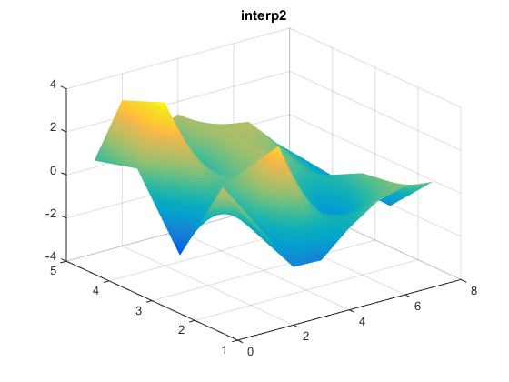
I've turned the edges off because they would be the edges of the high-res grid. We want to add the edges of the low-res grid. We'll have to do that in two steps.

First the column edges.

[x3,y3] = meshgrid(1:m,1:.1:n);
z3 = interp2(x,y,z, x3,y3);
c = surf(x3,y3,z3);
c.FaceColor = 'none';
c.MeshStyle = 'column';
hold on

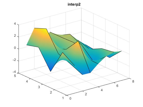
And then the row edges.

[x3,y3] = meshgrid(1:.1:m,1:n);
z3 = interp2(x,y,z, x3,y3);
r = surf(x3,y3,z3);
r.FaceColor = 'none';
r.MeshStyle = 'row';

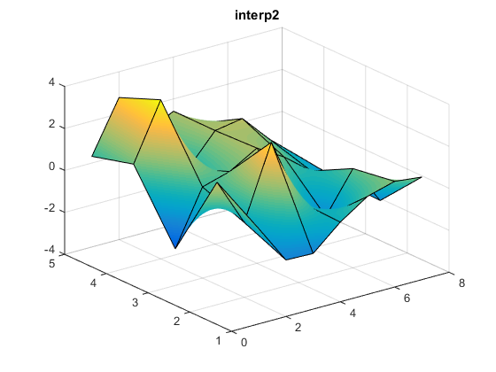
And finally we'll add the markers at the original data points.

m = surf(x,y,z);
m.FaceColor = 'none';
m.MeshStyle = 'none';
m.Marker = 's';
m.MarkerFaceColor = [.7 .2 .3];
m.MarkerEdgeColor = 'none';
hold off

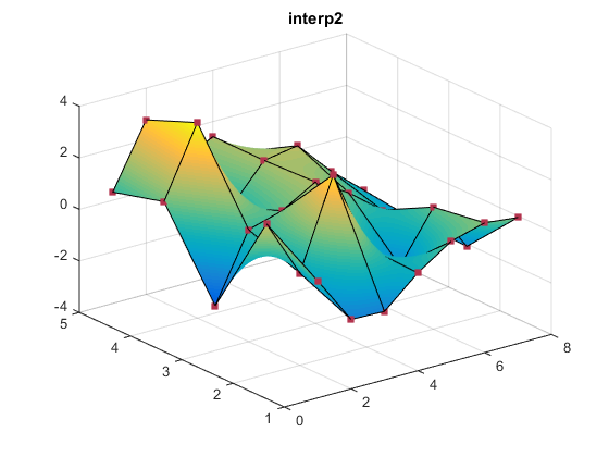
That looks pretty close to what surf did, doesn't it?

The interp2 function takes an argument named method that we didn't use before. We'd like to see what it looks like when we choose different values for method. We'll do that by converting those previous steps into the following function so that we can call it multiple times.

function interpsurf(z, method)
  if nargin < 2
    method = 'linear';
  end
  [n, m] = size(z);
  [x, y] = meshgrid(1:m,1:n);         % low-res grid
  [x2,y2] = meshgrid(1:.1:m,1:.1:n);  % high-res grid
  z2 = interp2(x,y,z, x2,y2, method); % interpolate up
  % Draw the faces with no edges using the high-res grid
  f = surf(x2,y2,z2);
  f.EdgeColor = 'none';
  f.FaceColor = 'interp';
  f.FaceLighting = 'gouraud';
  hold on
  % Add the column edges using a mix of low-res and high-res
  [x3,y3] = meshgrid(1:m,1:.1:n);
  z3 = interp2(x,y,z, x3,y3, method);
  c = surf(x3,y3,z3);
  c.FaceColor = 'none';
  c.MeshStyle = 'column';
  % Add the row edges
  [x3,y3] = meshgrid(1:.1:m,1:n);
  z3 = interp2(x,y,z, x3,y3, method);
  r = surf(x3,y3,z3);
  r.FaceColor = 'none';
  r.MeshStyle = 'row';
  % Add markers at the original points
  m = surf(x,y,z);
  m.FaceColor = 'none';
  m.EdgeColor = 'none';
  m.Marker = 's';
  m.MarkerFaceColor = [.7 .2 .3];
  m.MarkerEdgeColor = 'none';
  hold off

Now we can try the four different options for the method argument and compare the resulting surfaces.

f2 = figure('Position',[100 100 760 600]);
subplot(2,2,1)
interpsurf(z,'linear')
title linear
axis tight
subplot(2,2,2)
interpsurf(z,'spline')
title spline
axis tight
subplot(2,2,3)
interpsurf(z,'nearest')
title nearest
axis tight
subplot(2,2,4)
interpsurf(z,'cubic')
title cubic
axis tight

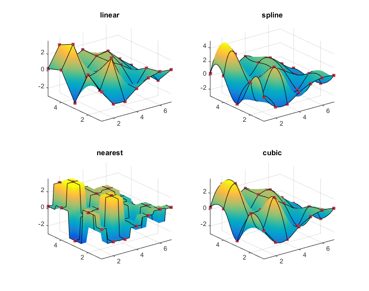
As you can see, all of these functions pass through the original points. But they behave quite differently in between those points. That's showing the difference between the various interpolation methods.

The different interpolation methods have some notable characteristics.

There's usually not one "right" choice for an interpolation function. You often need to strike a balance between boundedness, smoothness, and other characteristics of the interpolation function.

Of these, it looks like the linear option is the same as what surf did, but if we look closely we can see that there are actually some small differences.

Can you spot the differences?

The difference is that interp2 is doing something called bilinear interpolation, but surf is doing something called "piecewise linear" interpolation. These interpolation techniques are similar, but they're not quite the same.

The term bilinear interpolation means that it is actually the product of two linear equations. One is a linear interpolation in X.

$$f(x) = a_1 + a_2 x$$

The other equation is a linear interpolation in Y.

$$f(y) = b_1 + b_2 y$$

But the product of the two is not a linear equation. It is actually a quadratic equation which looks something like this:

$$f(x,y) = c_1 + c_2 x + c_3 y + c_4 x y$$

In the piecewise linear case, surf is actually breaking the 2x2 square into two triangles and then performing linear interpolation within the triangle using a linear equation.

The reason that surf uses piecewise linear is that modern graphics cards can evaluate linear equations very quickly, but they're not as good at the quadratic equation we encounter in bilinear interpolation. This means that piecewise linear has an important performance advantage over bilinear.

As we can see, this piecewise linear approach is very similar to the linear option. In fact, it is exactly the same as the linear option along the edges. It also has the boundedness property of the linear option. In general it's usually close enough to linear that the improved performance makes it worth using.

But it does have one important weakness. It is even less smooth than the linear option because it adds an extra crease along the diagonal of each 2x2 set of neighboring points where the two triangles meet. These diagonals also mean that surf's piecewise linear interpolation is anisotropic, rather than being isotropic like the bilinear interpolation that interp2 uses. This can be important in some cases.

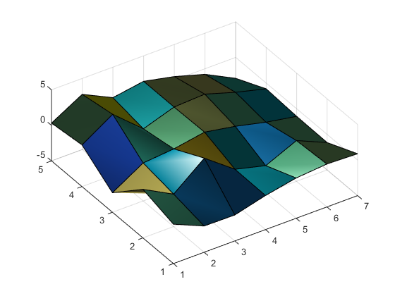
You can see one of the creases in the light blue square one up from the bottom in this picture.

delete(f2);
clf(f1);
surf(z)
h = light;
h.Style = 'local';
h.Position = [1.5 3 3];
view(-33.5,60)

It is important to recognize when surf's interpolation scheme is not the one which is appropriate for your purposes. When it's not, you'll want to use something like the interpsurf function we wrote today.

Get the MATLAB code

Published with MATLAB® R2014b