
Area Scaling
Last time we looked at how the performance of MATLAB's graphics system scales with the number of data points. Another interesting lens to look at performance scaling with is the way that performance scales with the number of pixels. This can actually show us a lot of interesting details of the balance of the compute and memory systems of our graphics card.
When we look at performance scaling through this lens, we'll keep coming up with charts that look something like this:
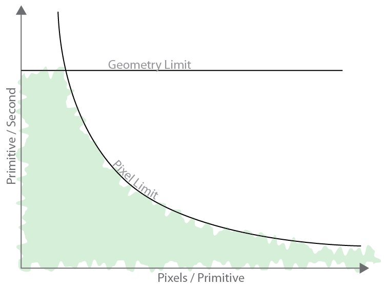
In this chart, the X axis is the size of the object we're drawing in pixels, and the Y axis is the number of objects we can draw per second. As you can see, I've sketched two curves on the chart. The one labeled "Pixel Limit" is a hyperbola which represents a constant number of pixels per second. The other curve is a horizontal line which I've labeled "Geometry Limit". These are also known as the "fill rate" and "setup rate". To a first order approximation, the "pixel limit" is a function of the details of the graphics card's memory system, and the "geometry limit" is a function of the graphics card's GPU. When we measure performance, we'll find that we always get numbers that are somewhere in the green shaded area. It isn't possible to cross over those two curves. In fact, as we'll see, it is usually pretty hard to get results up in that corner where the two curves meet. Real, measured data usually rounds off the corner between these two curves.
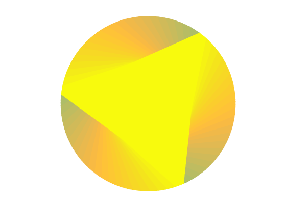
So let's collect some measurements and see how real data compares to this sketch. The following chunk of code creates 2,500 triangles and spins them around for 150 frames. It spins them using the hgtransform technique I described in this post.
ntri = 2500;
nframe = 150;
radii = linspace(0,1,75);
areas = (171.5*radii).^2 * 3 * sqrt(3) / 4;
seconds = zeros(1,length(radii));
for j=1:length(radii)
    rad = radii(j);
    cla
    axis square
    axis off
    xlim([-1 1])
    ylim([-1 1])
    g = hgtransform;
    theta = linspace(0,2*pi,ntri);
    v = [rad*cos(theta)', rad*sin(theta)'];
    x = 1:ntri;
    o1 = floor(ntri/3);
    o2 = floor(2*ntri/3);
    f = [x', 1+mod(x+o1,ntri)', 1+mod(x+o2,ntri)'];
    h = patch('Faces',f,'Vertices',v,'FaceVertexCData',x', ...
              'FaceColor','flat','EdgeColor','none', ...
              'Parent',g);
    drawnow
    t = nan(1,nframe);
    rotmat = makehgtform('zrotate',pi/20);
    for k=1:nframe
        tic
        set(g,'Matrix',get(g,'Matrix') * rotmat);
        drawnow
        t(k) = toc;
        if sum(t(1:k)) > 1.5
            break
        end
    end
    seconds(j) = median(t(isfinite(t)));
end
Now we can plot these results like so:
plot(areas,ntri./seconds)
xlabel('Pixels per triangle')
ylabel('Triangles per second')
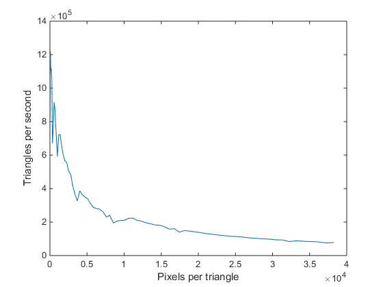
That looks kind of like the curve I sketched, but with a lot of noise for the small triangles. To make things clearer, lets add a "hyperbolic grid" with the following function:
function hyperbolicgrid
  radii = linspace(0,1,75);
  areas = (171.5*radii).^2 * 3 * sqrt(3) / 4;
  for j=1:8
    line(areas,j*1e9./areas,'Color',[.875 .875 .875], ...
         'HandleVisibility','off')
  end
cla
hold on
hyperbolicgrid
plot(areas,ntri./seconds)
xlabel('Pixels per triangle')
ylabel('Triangles per second')
xlim([0 inf])
ylim([0 5e5])
title('Performance Scaling')
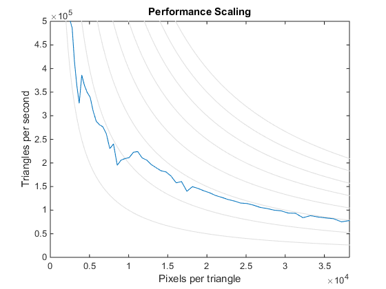
Now we can see that the curve doesn't actually follow one of the hyperbolas. The fill rate for small triangles is actually quite a bit lower than the fill rate for large triangles. This is something that you'll often see in real data. What's happening here is that the graphics card's memory system is very wide. That's part of the trick that makes a graphics card's memory system so fast. When we're drawing small triangles we're not touching enough neighboring pixels to take full advantage of the width of the memory system and so we lose some efficiency. But the details of shape of the pixel limit depend on your graphics card. In this case, I'm using a nVidia Quadro K600.
opengl info
                          Version: '4.4.0'
                           Vendor: 'NVIDIA Corporation'
                         Renderer: 'Quadro K600/PCIe/SSE2'
                   MaxTextureSize: 16384
                           Visual: 'Visual 0x07, (RGBA 32 bits (8 8 8 8), ...'
                         Software: 'false'
        SupportsGraphicsSmoothing: 1
    SupportsDepthPeelTransparency: 1
       SupportsAlignVertexCenters: 1
                       Extensions: {293x1 cell}
               MaxFrameBufferSize: 16384
I've run that code above with a number of different settings and we can use these results to see how those settings affect graphics performance. For example, how does the SortMethod property affect performance? The default was childorder because those triangles are all at Z=0. When I switch to
set(gca,'SortMethod','depthsort')
I get a different results.
load r2014b_results
load depthsort_results
cla
hold on
hyperbolicgrid
plot(areas,ntri./r2014b_results)
plot(areas,ntri./depthsort_results)
xlabel('Pixels per triangle')
ylabel('Triangles per second')
xlim([0 inf])
ylim([0 5e5])
legend('childorder','depthsort')
title('SortMethod')
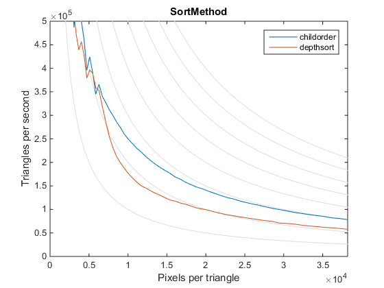
You can see that the pixel limit is lower for large triangles, but for small triangles the difference is pretty negligible because of those efficiency issues. You can also see that the depthsort curve is a little unusual because it doesn't "droop off" on the left side. This is actually a result of some interesting optimizations that modern graphics cards use to accelerate depthsorting for small triangles.
What about software opengl? How does it's performance compare to the hardware?
load r2014b_results
load sw_results
cla
hold on
hyperbolicgrid
plot(areas,ntri./r2014b_results)
plot(areas,ntri./sw_results)
xlabel('Pixels per triangle')
ylabel('Triangles per second')
xlim([0 inf])
ylim([0 5e5])
legend('hardware','software')
title('Hardware vs. Software')

We can see that using software opengl affects both limits, and quite substantially. The difference between these two curves will, of course, depend on what type of graphics card your system has. But it does highlight the importance of making sure that your graphics card drivers are up to date so that MATLAB can use hardware OpenGL.
And finally, how do different versions of MATLAB compare?
load r2014b_results
load r2014a_results
cla
hold on
hyperbolicgrid
plot(areas,ntri./r2014b_results)
plot(areas,ntri./r2014a_results)
xlabel('Pixels per triangle')
ylabel('Triangles per second')
xlim([0 inf])
ylim([0 5e5])
legend('R2014b','R2014a')
title('R2014b vs. R2014a')
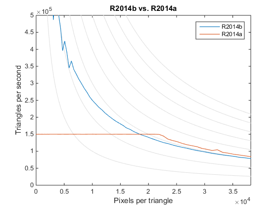
That's interesting, isn't it? It turns out that the old graphics system in R2014a actually had a slightly higher pixel limit than the current version. That's because the new one has added features such as GraphicsSmoothing which incur costs per pixel. But the geometry limit of the old version was only 150,000 triangles per second. That's much, much lower than the geometry limit of the new graphics system. That's because the old graphics system was designed when graphics cards had much lower geometry limits and it had some architectural isses feeding geometry to the card quickly. This bottleneck is one of the things we wanted to make sure we fixed when we were designing a new graphics system for MATLAB.
I should mention here that there are per-pixel costs in initializing the window and in swapping the completed picture onto the screen. This means that to get the most accurate versions of these curves we should really scale the size of the figure window rather than just the size of the triangles we're drawing into the figure window. But doing that made the code a bit more complex, and it really doesn't have a very large effect in this particular case, so I haven't done that here. But you might find that useful if you try to do this sort of area scaling analysis.
As you can see, this view of performance scaling is a powerful one for understanding the bottlenecks in your graphics system. This is often the first technique I try when I'm trying to understand a new graphics performance issue.
- Category:
- Performance

