Steve on Image Processing

Today I'm introducing a series on computing the location of the US continental divide. (I was inspired to tackle this topic by Brian Hayes' blog post on the divide; thanks very much to Mike and Ned for sending me the link.)

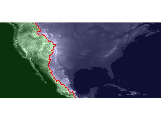
The series will start with importing global elevation data for Earth, and it will finish with this visualization of the Atlantic and Pacific catchment basins for the continental US:

My regular blog readers might be happy to know that this time I've planned and written out the whole series in advance. See below for the series summary.

In this first post, I'll tackle data import and display.

The data for this project comes from the Global Land One-km Base Elevation Project, available from the National Geophysical Data Center. The global elevation data set is available online in the form of 16 tiles, labeled A through P. Tile E and and tile F cover the continental United States, Central America, and portions of Canada and South America.

After you've downloaded and uncompressed the files, you have to figure out how to import them. As it turns out, these files are not in a structured format, such as TIFF or HDF, that can be read automatically. Instead, you need to poke around the data documentation on the web to find out how to read the files. This is fairly common with scientific data sources. The documentation for this data set includes a section called "Data Format & Importing GLOBE Data." By perusing this section I found that the files I downloaded contain 16-bit signed integers organized in a raster of 6000 rows and 10800 columns, stored by row. There are no header bytes, and the integers are stored using little-endian byte order.

The appropriate MATLAB function to use is multibandread.

data_size = [6000 10800 1];  % The data has 1 band.
precision = 'int16=>int16';  % Read 16-bit signed ints into a int16 array.
header_bytes = 0;
interleave = 'bsq';          % Band sequential. Not critical for 1 band.
byte_order = 'ieee-le';

E = multibandread('e10g', data_size, precision, header_bytes, ...
    interleave, byte_order);
F = multibandread('f10g', data_size, precision, header_bytes, ...
    interleave, byte_order);

dem = [E, F];  % dem stands for "Digital Elevation Model"

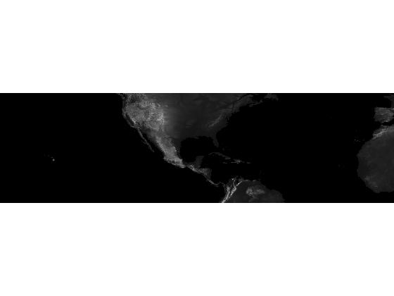
Next I'll use imshow, using some optional inputs, to display the digital elevation model as an image.

imshow(dem, [], 'InitialMagnification', 'fit')

About those optional inputs: When displaying gridded data as an image, it is often useful to control the black-to-white display range. If you supply a vector as the second input to imshow, like this:

   imshow(dem, [a b])

then imshow uses [a b] as the image display range. A value of a gets displayed as black, a value of b gets displayed as white, and values in-between are displayed as shades of gray.

For the special case where the second input is empty:

   imshow(dem, [])

imshow uses the data range as the display range. That is, imshow(dem, []) is equivalent to imshow(dem, [min(dem(:)), max(dem(:))]).

The other optional inputs, 'InitialMagnification', 'fit', tell imshow to magnify or shrink the image display as needed to fit nicely within the current figure window. I'm using that option here so that my image displays will fit in the column for this blog post.

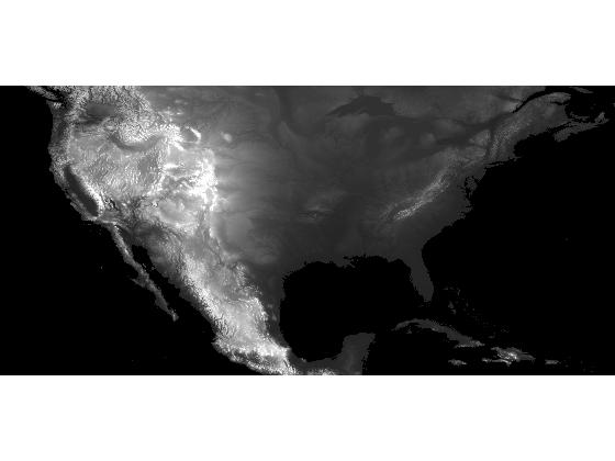
For this data, the autoscaling provided by the imshow(dem, []) syntax has given us an image display that is too dark, particularly on the eastern part of the continent. Let's set a white level that's lower than the data maximum; that will have the effect of brightening the image.

min(dem(:))

ans =

   -500

max(dem(:))

ans =

   6085

display_range = [-500 3000];
imshow(dem, display_range, 'InitialMagnification', 'fit')

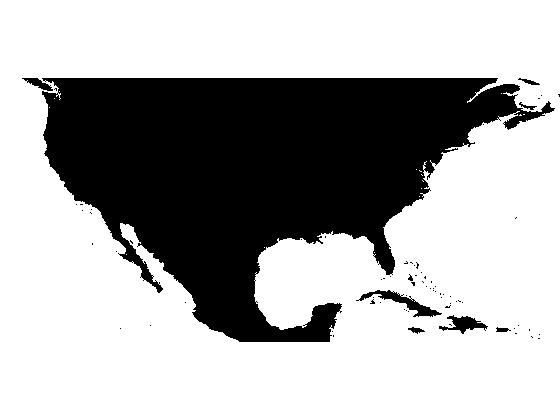
Next I'll crop the image. The Image Processing Toolbox has interactive cropping tools (imcrop, imtool), but I can't use those here.

dem_cropped = dem(1:4000, 6000:14500);
imshow(dem_cropped, display_range, 'InitialMagnification', 'fit')

Finally, I'll save dem_cropped to a MAT-file for use in the rest of the series.

save continental_divide dem_cropped

About this Series

This series explores the problem of computing the location of the continental divide for the United States. The divide separates the Atlantic and Pacific Ocean catchment basins for the North American continent.

As an algorithm development problem, computing the divide lets us explore aspects of data import and visualization, manipulating binary image masks, label matrices, regional minima, and the watershed transform.

Data credit: GLOBE Task Team and others (Hastings, David A., Paula K. Dunbar, Gerald M. Elphingstone, Mark Bootz, Hiroshi Murakami, Hiroshi Maruyama, Hiroshi Masaharu, Peter Holland, John Payne, Nevin A. Bryant, Thomas L. Logan, J.-P. Muller, Gunter Schreier, and John S. MacDonald), eds., 1999. The Global Land One-kilometer Base Elevation (GLOBE) Digital Elevation Model, Version 1.0. National Oceanic and Atmospheric Administration, National Geophysical Data Center, 325 Broadway, Boulder, Colorado 80305-3328, U.S.A. Digital data base on the World Wide Web (URL: http://www.ngdc.noaa.gov/mgg/topo/globe.html) and CD-ROMs.

Get the MATLAB code

Published with MATLAB® 7.8