
a* and b*
Note added 27-Apr-2021: See the updated discussion of this topic in the 27-Apr-2021 post, "Plotting a* and b* colors."
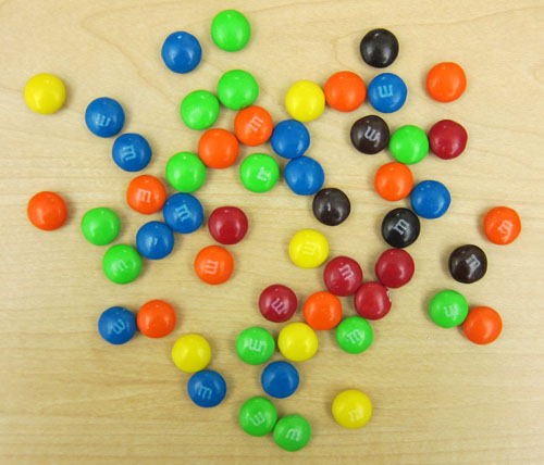
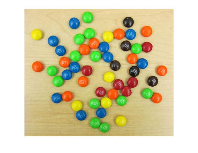
Last week I showed how to compute a two-dimensional histogram. Specifically, I computed the two-dimensional histogram of the a*-b* values of this image:
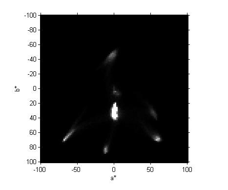
This was the result:
Blog reader Vanessa naturally wanted to know what this all means. (And blog reader Cmac gave a pretty good answer.)
Let me elaborate a bit. By L*a*b* I refer to the CIE 1976 L*, a*, b* color space. Here's a description of the three dimensions (from the Wikipedia article):
"The three coordinates of CIELAB represent the lightness of the color (L* = 0 yields black and L* = 100 indicates diffuse white; specular white may be higher), its position between red/magenta and green (a*, negative values indicate green while positive values indicate magenta) and its position between yellow and blue (b*, negative values indicate blue and positive values indicate yellow). The asterisk after L, a and b are part of the full name, since they represent L*, a* and b*, to distinguish them from Hunter's L, a and b, [an earlier color space]."
Bright spots in the two-dimensional histogram indicate that a relatively large number of pixels in the original image have the corresponding a* and b* values.
Consider, for example, the lowest bright spot on the two-dimensional histogram. By using impixelinfo and my mouse I was able to see that the a* and b* values for this spot are about -12 and 85. What color is that? To convert back to RGB values that we can display I have to pick some value for L*, whose natural range is 0 to 100. I'll pick 90, a fairly bright value. Then I use applycform to convert from L*a*b* to sRGB.
lab = [90 -12 85];
rgb = applycform(lab, makecform('lab2srgb'))
rgb =

    0.9297    0.9066    0.0971
How can we look at this color? There are a lot of different ways. One procedure is to display a 1-by-1 indexed image with a one-color colormap.
image(1)
colormap(rgb)
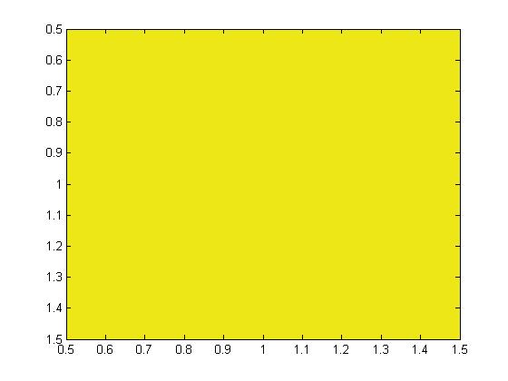
Looks like we found yellow! How about some of the other colors? The left-most bright spot is at about (-68,70). The right-most spot is at about (60,70), and the top-most spot is at about (-4,-47).
lab = [90 -68 70; 90 60 70; 90 -4 -47];
rgb = applycform(lab, makecform('lab2srgb'))
rgb =

    0.3737    1.0000    0.2844
    1.0000    0.6832    0.3652
    0.6637    0.9077    1.0000
image([1 2 3])
colormap(rgb)
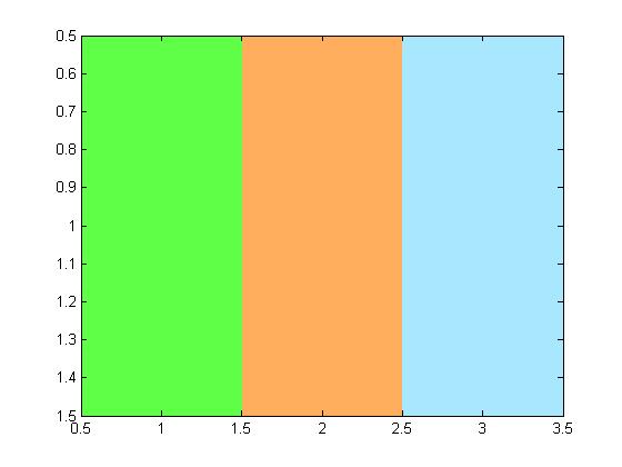
The two colors on the right don't look that much like any of our M&Ms. Maybe I guessed wrong about L*.
lab(:,1) = 50
lab =

    50   -68    70
    50    60    70
    50    -4   -47
rgb = applycform(lab, makecform('lab2srgb'));
image([1 2 3])
colormap(rgb)
That's better. We found our green, red, and blue M&M colors.
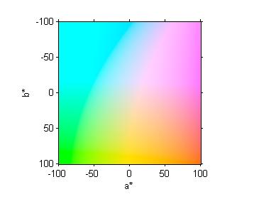
Note added 27-Apr-2021: The following explanation fails to note that many of the colors in the a*-b* plane are actually out of gamut. See the updated discussion of this topic in the 27-Apr-2021 post, "Plotting a* and b* colors."
Here's a crude way to visualize all the colors of the a*-b* plane. We make an "image" containing L*a*b* values and then convert the whole thing to RGB.
[a,b] = meshgrid(-100:100);
L = 90*ones(size(a));
lab = cat(3, L, a, b);
rgb = applycform(lab, makecform('lab2srgb'));
imshow(rgb, 'XData',[-100 100], 'YData', [-100 100])
xlabel('a*')
ylabel('b*')
axis on
I will continue for a while longer to use this image as an excuse for a pseudorandom walk through some image processing computational and visualization techniques. We've looked at color-space conversion, two-dimensional histograms, and ways to show individual color patches.
I think that next time I'll start to look at segmentation based on color.
In the meantime, Happy New Year everyone!


Comments
To leave a comment, please click here to sign in to your MathWorks Account or create a new one.