
Splines and Pchips
MATLAB has two different functions for piecewise cubic interpolation, spline and pchip. Why are there two? How do they compare?

 If we piece together enough cubics like these to produce a piecewise cubic that interpolates many data points, we have a PCHIP. We could even mix colors and still have a PCHIP. Clearly, we have to be specific when it comes to specifying the slopes.
One possibility that might occur to you briefly is to use the slopes of the lines connecting the end points of each segment. But this choice just produces zeros for the coefficients of the cubics and leads back to the piecewise linear interpolant. After all, a linear function is a degenerate cubic. This illustrates the fact that the PCHIP family includes many functions.
If we piece together enough cubics like these to produce a piecewise cubic that interpolates many data points, we have a PCHIP. We could even mix colors and still have a PCHIP. Clearly, we have to be specific when it comes to specifying the slopes.
One possibility that might occur to you briefly is to use the slopes of the lines connecting the end points of each segment. But this choice just produces zeros for the coefficients of the cubics and leads back to the piecewise linear interpolant. After all, a linear function is a degenerate cubic. This illustrates the fact that the PCHIP family includes many functions.
Contents
Data
Here is the data that I will use in this post.x = 1:6 y = [16 18 21 17 15 12]
x =

     1     2     3     4     5     6


y =

    16    18    21    17    15    12
Here is a plot of the data.
set(0,'defaultlinelinewidth',2)
clf
plot(x,y,'-o')
axis([0 7 7.5 25.5])
title('plip')
plip
With line type '-o', the MATLAB plot command plots six 'o's at the six data points and draws straight lines between the points. So I added the title plip because this is a graph of the piecewise linear interpolating polynomial. There is a different linear function between each pair of points. Since we want the function to go through the data points, that is interpolate the data, and since two points determine a line, the plip function is unique.The PCHIP Family
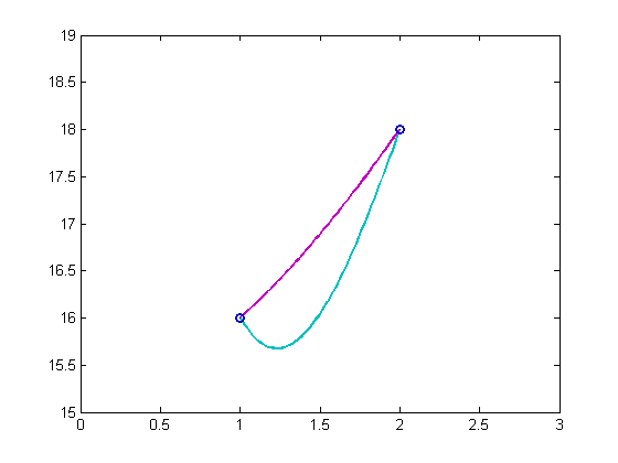
A PCHIP, a Piecewise Cubic Hermite Interpolating Polynomial, is any piecewise cubic polynomial that interpolates the given data, AND has specified derivatives at the interpolation points. Just as two points determine a linear function, two points and two given slopes determine a cubic. The data points are known as "knots". We have the y-values at the knots, so in order to get a particular PCHIP, we have to somehow specify the values of the derivative, y', at the knots. Consider these two cubic polynomials in $x$ on the interval $1 \le x \le 2$ . These functions are formed by adding cubic terms that vanish at the end points to the linear interpolatant. I'll tell you later where the coefficients of the cubics come from. $$ s(x) = 16 + 2(x-1) + \textstyle{\frac{49}{18}}(x-1)^2(x-2) - \textstyle{\frac{89}{18}}(x-1)(x-2)^2 $$ $$ p(x) = 16 + 2(x-1) + \textstyle{\frac{2}{5}}(x-1)^2(x-2) - \textstyle{\frac{1}{2}}(x-1)(x-2)^2 $$ These functions interpolate the same values at the ends. $$ s(1) = 16, \ \ \ s(2) = 18 $$ $$ p(1) = 16, \ \ \ p(2) = 18 $$ But they have different first derivatives at the ends. In particular, $s'(1)$ is negative and $p'(1)$ is positive. $$ s'(1) = - \textstyle{\frac{53}{18}}, \ s'(2) = \textstyle{\frac{85}{18}} $$ $$ p'(1) = \textstyle{\frac{3}{2}}, \ \ \ p'(2) = \textstyle{\frac{12}{5}} $$ Here's a plot of these two cubic polynomials. The magenta cubic, which is $p(x)$, just climbs steadily from its initial value to its final value. On the other hand, the cyan cubic, which is $s(x)$, starts off heading in the wrong direction, then has to hurry to catch up.x = 1:1/64:2; s = 16 + 2*(x-1) + (49/18)*(x-1).^2.*(x-2) - (89/18)*(x-1).*(x-2).^2; p = 16 + 2*(x-1) + (2/5)*(x-1).^2.*(x-2) - (1/2)*(x-1).*(x-2).^2; clf axis([0 3 15 19]) box on line(x,s,'color',[0 3/4 3/4]) line(x,p,'color',[3/4 0 3/4]) line(x(1),s(1),'marker','o','color',[0 0 3/4]) line(x(end),s(end),'marker','o','color',[0 0 3/4])
If we piece together enough cubics like these to produce a piecewise cubic that interpolates many data points, we have a PCHIP. We could even mix colors and still have a PCHIP. Clearly, we have to be specific when it comes to specifying the slopes.
One possibility that might occur to you briefly is to use the slopes of the lines connecting the end points of each segment. But this choice just produces zeros for the coefficients of the cubics and leads back to the piecewise linear interpolant. After all, a linear function is a degenerate cubic. This illustrates the fact that the PCHIP family includes many functions.
spline
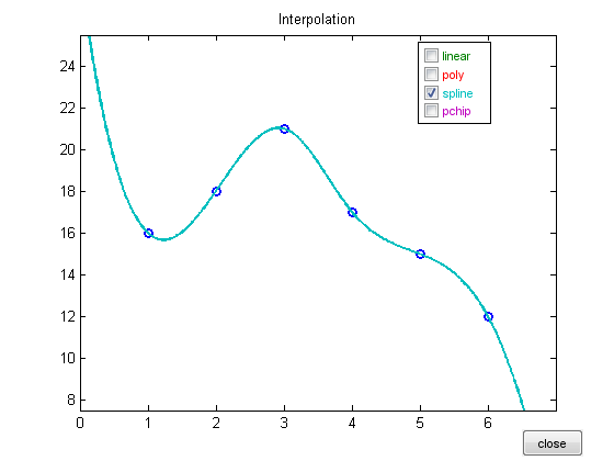
By far, the most famous member of the PCHIP family is the piecewise cubic spline. All PCHIPs are continuous and have a continuous first derivative. A spline is a PCHIP that is exceptionally smooth, in the sense that its second derivative, and consequently its curvature, also varies continuously. The function derives its name from the flexible wood or plastic strip used to draw smooth curves. Starting about 50 years ago, Carl de Boor developed much of the basic theory of splines. He wrote a widely adopted package of Fortran software, and a widely cited book, for computations involving splines. Later, Carl authored the MATLAB Spline Toolbox. Today, the Spline Toolbox is part of the Curve Fitting Toolbox. When Carl began the development of splines, he was with General Motors Research in Michigan. GM was just starting to use numerically controlled machine tools. It is essential that automobile parts have smooth edges and surfaces. If the hood of a car, say, does not have continuously varying curvature, you can see wrinkles in the reflections in the show room. In the automobile industry, a discontinuous second derivative is known as a "dent". The requirement of a continuous second derivative leads to a set of simultaneous linear equations relating the slopes at the interior knots. The two end points need special treatment, and the default treatment has changed over the years. We now choose the coefficients so that the third derivative does not have a jump at the first and last interior knots. Single cubic pieces interpolate the first three, and the last three, data points. This is known as the "not-a-knot" condition. It adds two more equations to set of equations at the interior points. If there are n knots, this gives a well-conditioned, almost symmetric, tridiagonal $n$ -by- $n$ linear system to solve for the slopes. The system can be solved by the sparse backslash operator in MATLAB, or by a custom, non-pivoting tridiagonal solver. (Other end conditions for splines are available in the Curve Fitting Toolbox.) As you probably realized, the cyan function $s(x)$ introduced above, is one piece of the spline interpolating our sample data. Here is a graph of the entire function, produced by interpgui from NCM, Numerical Computing with MATLAB.x = 1:6; y = [16 18 21 17 15 12]; interpgui(x,y,3)
sppchip
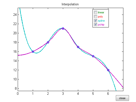
I just made up that name, sppchip. It stands for shape preserving piecewise cubic Hermite interpolating polynomial. The actual name of the MATLAB function is just pchip. This function is not as smooth as spline. There may well be jumps in the second derivative. Instead, the function is designed so that it never locally overshoots the data. The slope at each interior point is taken to be a weighted harmonic mean of the slopes of the piecewise linear interpolant. One-sided slope conditions are imposed at the two end points. The pchip slopes can be computed without solving a linear system. pchip was originally developed by Fred Fritsch and his colleagues at Lawrence Livermore Laboratory around 1980. They described it as "visually pleasing". Dave Kahaner, Steve Nash and I included some of Fred's Fortran subroutines in our 1989 book, Numerical Methods and Software. We made pchip part of MATLAB in the early '90s. Here is a comparison of spline and pchip on our data. In this case the spline overshoot on the first subinterval is caused by the not-a-knot end condition. But with more data points, or rapidly varying data points, interior overshoots are possible with spline.interpgui(x,y,3:4)
spline vs. pchip
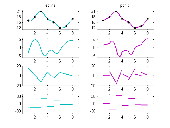
Here are eight subplots comparing spline and pchip on a slightly larger data set. The first two plots show the functions $s(x)$ and $p(x)$. The difference between the functions on the interior intervals is barely noticeable. The next two plots show the first derivatives. You can see that the first derivative of spline, $s'(x)$, is smooth, while the first derivative of pchip, $p'(x)$, is continuous, but shows "kinks". The third pair of plots are the second derivatives. The spline second derivative $s''(x)$ is continuous, while the pchip second derivative $p''(x)$ has jumps at the knots. The final pair are the third derivatives. Because both functions are piecewise cubics, their third derivatives, $s'''(x)$ and $p'''(x)$, are piecewise constant. The fact that $s'''(x)$ takes on the same values in the first two intervals and the last two intervals reflects the "not-a-knot" spline end conditions.splinevspchip
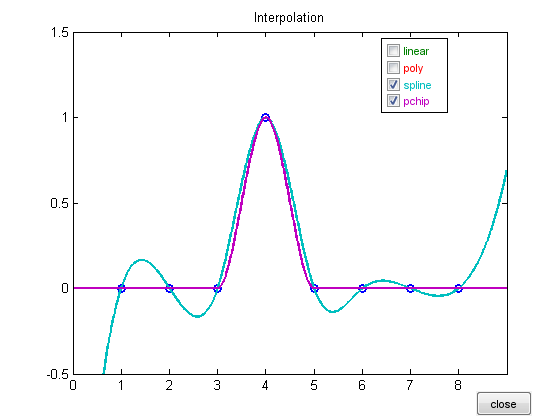
Locality
pchip is local. The behavior of pchip on a particular subinterval is determined by only four points, the two data points on either side of that interval. pchip is unaware of the data farther away. spline is global. The behavior of spline on a particular subinterval is determined by all of the data, although the sensitivity to data far away is less than to nearby data. Both behaviors have their advantages and disadvantages. Here is the response to a unit impulse. You can see that the support of pchip is confined to the two intervals surrounding the impulse, while the support of spline extends over the entire domain. (There is an elegant set of basis functions for cubic splines known as B-splines that do have compact support.)x = 1:8; y = zeros(1,8); y(4) = 1; interpgui(x,y,3:4)
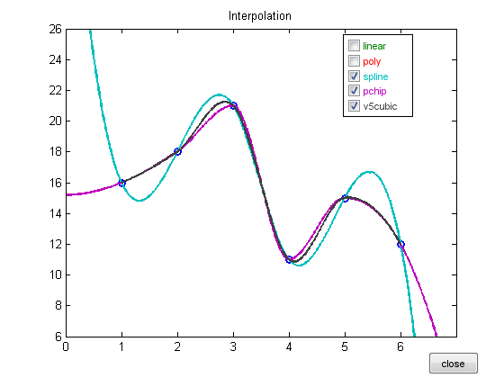
interp1
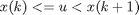
The interp1 function in MATLAB, has several method options. The 'linear', 'spline', and 'pchip' options are the same interpolants we have been discussing here. We decided years ago to make the 'cubic' option the same as 'pchip' because we thought the monotonicity property of pchip was generally more desirable than the smoothness property of spline. The 'v5cubic' option is yet another member of the PCHIP family, which has been retained for compatibility with version 5 of MATLAB. It requires the x's to be equally spaced. The slope of the v5 cubic at point $x_n$ is $(y_{n+1} - y_{n-1})/2$. The resulting piecewise cubic does not have a continuous second derivative and it does not always preserve shape. Because the abscissa are equally spaced, the v5 cubic can be evaluated quickly by a convolution operation. Here is our example data, modified slightly to exaggerate behavior, and interpgui modified to include the 'v5cubic' option of interp1. The v5 cubic is the black curve between spline and pchip.x = 1:6; y = [16 18 21 11 15 12]; interpgui_with_v5cubic(x,y,3:5)
Resources
A extensive collection of tools for curve and surface fitting, by splines and many other functions, is available in the Curve Fitting Toolbox.doc curvefit
"NCM", Numerical Computing with MATLAB, has more mathematical details. NCM is available online. Here is the interpolation chapter. Here is interpgui. SIAM publishes a print edition.
Here are the script splinevspchip.m and the modified version of interpgui interpgui_with_v5cubic.m that I used in this post.
- カテゴリ:
- Algorithms


See Also
-
Interpolation in MATLAB
Blogs
-
-


コメント
コメントを残すには、ここ をクリックして MathWorks アカウントにサインインするか新しい MathWorks アカウントを作成します。