I have been interested in the computation of the matrix exponential, $e^A$, for a long time. A recent query from a user provides a provocative example.

Contents

Nineteen Dubious Ways

In 1978, Charlie Van Loan and I published a paper in SIAM Review entitled "Nineteen Dubious Ways to Compute the Exponential of a Matrix". The paper does not pick a "best of the 19", but cautiously suggests that the "scaling and squaring" algorithm might be OK. This was about the time I was tinkering with the first MATLAB and consequently every version of MATLAB has had an expm function, based on scaling and squaring. The SIAM Review paper proved to be very popular and in 2003 we published a followup, "Nineteen Dubious Ways ..., Twenty-Five Years Later". A PDF is available from Charlie's web site.

Our colleague Nick Higham reconsided the matrix exponential in 2005. Nick did a careful error analysis of scaling and squaring, improved the efficiency of the algorithm, and wrote a paper for the SIAM Journal on Numerical Analysis, "The scaling and squaring method for the matrix exponential revisited". A PDF is available from the University of Manchester's web site. The current version of expm in MATLAB is Nick's implementation of scaling and squaring.

A more recent review of Nick's work on the matrix exponential is provided by these slides for a talk he gave at a meeting in Rome in 2008.

A Query from a User

A few weeks ago, MathWorks Tech Support received a query from a user about the following matrix. Note that the elements of A range over 18 orders of magnitude.

format long g
a = 2e10;
b = 4e8/6;
c = 200/3;
d = 3;
e = 1e-8;
A = [0 e 0; -(a+b) -d a; c 0 -c]

A =

                         0                     1e-08                         0
         -20066666666.6667                        -3               20000000000
          66.6666666666667                         0         -66.6666666666667

The computed matrix exponential has huge elements.

E = expm(A)

E =

       1.7465684381715e+17         -923050477.783131     -1.73117355055901e+17
     -3.07408665108297e+25      1.62463553675545e+17      3.04699053651329e+25
      1.09189154376804e+17         -577057840.468934     -1.08226721572342e+17

The report claimed that the right answer, obtained from a MATLAB competitor, differs from E by many orders of magnitude.

[  0.446849, 1.54044*10^-9, 0.462811,
  -5.74307*10^6, -0.015283, -4.52654*10^6
   0.447723, 1.5427*10^-9, 0.463481]

ans =

                  0.446849               1.54044e-09                  0.462811
                  -5743070                 -0.015283                  -4526540
                  0.447723                1.5427e-09                  0.463481

Symbolic

Let's generate the symbolic representation of A.

a = sym(2e10);
b = sym(4e8)/6;
c = sym(200)/3;
d = sym(3);
e = sym(1e-8);
S = [0 e 0; -(a+b) -d a; c 0 -c]

 
S =
 
[              0, 1/100000000,           0]
[ -60200000000/3,          -3, 20000000000]
[          200/3,           0,      -200/3]
 

Now have the Symbolic Toolbox compute the matrix exponential, then convert the result to floating point. We can regard this as the "right answer". We see that it agrees with the user's expectations.

X = real(double(expm(S)))

X =

         0.446849468283175      1.54044157383952e-09         0.462811453558774
         -5743067.77947947       -0.0152830038686819         -4526542.71278401
         0.447722977849494      1.54270484519591e-09         0.463480648837651

Classic MATLAB

I ran my old Fortran MATLAB from 1980. Here is the output. It got the right answer.

% <>
% A = <0 e 0; -(a+b) -d a; c 0 -c>
%
%  A     =
%
%     0.000000000000000D+00   1.000000000000000D-08   0.000000000000000D+00
%    -2.006666666666667D+10  -3.000000000000000D+00   2.000000000000000D+10
%     6.666666666666667D+01   0.000000000000000D+00  -6.666666666666667D+01
%
% <>
% exp(A)
%
%  ANS   =
%
%     4.468494682831735D-01   1.540441573839520D-09   4.628114535587735D-01
%    -5.743067779479621D+06  -1.528300386868247D-02  -4.526542712784168D+06
%     4.477229778494929D-01   1.542704845195912D-09   4.634806488376499D-01

The Three Demos

In addition to expm, MATLAB has for many years provided three demo functions that illustrate popular methods for computing $e^A$. The function expmdemo1 is a MATLAB implementation of the scaling and squaring algorithm that was used in the builtin expm before Higham's improvements. The function expmdemo2 implements the Taylor power series that is often the definition of $e^A$, but which is one of the worst of the nineteen ways because it is slow and numerically unreliable. The function expmdemo3 uses eigenvalues and eigenvectors, which is OK only if the eigenvector matrix is well conditioned. (MATLAB also has a function expm1, which computes the scalar function $e^x\!-\!1$ without computing $e^x$. The m in the name is for minus, not matrix. This function has nothing to do with the matrix exponential.)

Let's see what the three demo functions do with our example.

%  Scaling and squaring
E1 = expmdemo1(A)

E1 =

         0.446848323199335      1.54043901480671e-09         0.462810666904014
         -5743177.01871262       -0.0152833835375292         -4526656.46142213
         0.447721814330828      1.54270222301338e-09          0.46347984316225

%  Taylor series
E2 = expmdemo2(A)

E2 =

         -3627968682.81884         0.502451507654604         -3062655286.68657
     -1.67974375988037e+19          3498209047.28622     -2.27506724048955e+19
           15580992163.692          7.53393732504015          4987630142.66227

%  Eigenvalues and eigenvectors
E3 = expmdemo3(A)

E3 =

         0.446849468283181      1.54044157383954e-09         0.462811453558778
         -5743067.77947891         -0.01528300386868         -4526542.71278343
           0.4477229778495      1.54270484519593e-09         0.463480648837654

You can see that both eigdemo1, the outdated scaling and squaring, and eigdemo3, eigenvectors, get the right answer, while eigdemo2, Taylor series, blows up.

Scaling, Squaring, and Pade Approximations

In outline, the scaling and squaring algorithm for computing $e^A$ is:

We have two implementations of scaling and squaring, the outdated one in expmdemo1 and the current one in expm. It turns out that, for this matrix, the old implementation decides the scale factor should be 2^37 while the current implementation chooses 2^32. Using the new scale factor will save five matrix multiplications in the unscaling by repeated squaring.

The key to the comparison of these two implementations lies in the eigenvalues of the Pade approximants.

P = expmdemo1(A/2^37);
e = eig(P)

P = expm(A/2^32);
e = eig(P)

e =

         0.999999999539043
         0.999999999954888
         0.999999999999176


e =

         0.999999974526488
          1.00000000930672
         0.999999999946262

In this case, the old code produces eigenvalues that are less than one. Powers of these eigenvalues, and hence powers of P, remain bounded. But the current code happens to produce an eigenvalue slightly larger than one. The powers of e and of P blow up.

e.^(2^32)

ans =

      3.05317714952674e-48
      2.28895048607366e+17
         0.793896973586281

Balancing

One cure, at least in this instance, is balancing. Balancing is a diagonal similarity transformation that tries to make the matrix closer to symmetric by making the row norms equal to the column norms. This may improve the accuracy of computed eigenvalues, but seriously alter the eigenvectors. The MATLAB documentation has a good discussion of the effect of balancing on eigenvectors.

% doc balance

Balancing the Exponential

Balancing can have sometimes have a beneficial effect in the computation of $e^A$. For the example in this blog the elements of the diagonal similarity transform are powers of 2 that vary over a wide range.

[T,B] = balance(A);
T
log2T = diag(log2(diag(T)))

T =

       9.5367431640625e-07                         0                         0
                         0                      2048                         0
                         0                         0       1.9073486328125e-06


log2T =

   -20     0     0
     0    11     0
     0     0   -19

In the balanced matrix $B = T^{-1} A T$, the tiny element $a_{1,2}=10^{-8}$ has been magnified to be comparable with the other elements.

B

B =

                         0               21.47483648                         0
          -9.3442698319753                        -3          18.6264514923096
          33.3333333333333                         0         -66.6666666666667

Computing the $e^B$ presents no difficulties. The final result obtained by reversing the scaling is what we have come to expect for this example.

M = T*expm(B)/T

M =

         0.446849468283175      1.54044157383952e-09         0.462811453558774
         -5743067.77947947       -0.0152830038686819           -4526542.712784
         0.447722977849495      1.54270484519591e-09          0.46348064883765

Condition

Nick Higham has contributed his Matrix Function Toolbox to MATLAB Central. The Toolbox has many useful functions, including expm_cond, which computes the condition number of the matrix exponential function. Balancing improves the conditioning of this example by 16 orders of magnitude.

addpath('../../MFToolbox')
expm_cond(A)
expm_cond(B)

ans =

      3.16119437847582e+18


ans =

          238.744549689702

Should We Use Balancing?

Bob Ward, in the original 1977 paper on scaling and squaring, recommended balancing. Nick Higham includes balancing in the pseudocode algorithm in his 2005 paper, but in recent email with me he was reluctant to recommend it. I am also reluctant to draw any conclusions from this one case. Its scaling is too bizarre. Besides, there is a better solution, avoid overscaling.

Overscaling

In 2009 Nick Higham's Ph. D. Student, Awad H. Al-Mohy, wrote a dissertation entitled "A New Scaling and Squaring Algorithm for the Matrix Exponential". The dissertation described a MATLAB function expm_new. A PDF of the dissertation and a zip file with the code are available from the University of Manchester's web site.

If $A$ is not a normal matrix, then the norm of the power, $||A^k||$, can grow much more slowly than the power of the norm, $||A||^k$. As a result, it is possible to suffer significant roundoff error in the repeated squaring. The choice of the scale factor $2^s$ involves a delicate compromise between the accuracy of the Pade approximation and the number of required squarings.

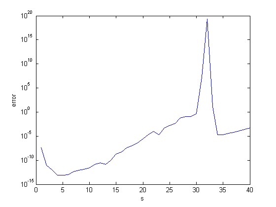
Here is one experiment with our example and various choices of $s$. The function padexpm is the order 13 Pade approximation taken from expm. We see that $s = 32$, which is the choice made by expm, is the worst possible choice. The old choice, $s = 37$, is much better. These large values of $s$ result from the fact that this particular matrix has a large norm. For this example, values of $s$ less than 10 are much better.

warning('off','MATLAB:nearlySingularMatrix')
err = zeros(40,1);
for s = 1:40
   P = padexpm(A/2^s);
   for k = 1:s
      P = P*P;
   end
   err(s) = norm((P-X)./X,inf);
end
semilogy(err)
xlabel('s')
ylabel('error')

expm_new

So how does the latest expm from Manchester do on this example? It chooses $s = 8$ and does a fine job.

expm_new(A)

ans =

         0.446849468283145      1.54044157383964e-09          0.46281145355881
         -5743067.77947979       -0.0152830038686872         -4526542.71278561
         0.447722977849464      1.54270484519604e-09         0.463480648837687

What Did I Learn?

This example is an extreme outlier, but it is instructive. The condition number of the problem is terrible. Small changes in the data might make huge changes in the result, but I haven't investigated that. The computed result might be the exact result for some matrix near the given one, but I haven't pursued that. The current version of expm in MATLAB computed an awful result, but it was sort of unlucky. We have seen at least half a dozen other functions, including classic MATLAB and expm with balancing, that get the right answer. It looks like expm_new should find its way into MATLAB.

Get the MATLAB code

Published with MATLAB® 7.14

Published with MATLAB® 7.14