
Floating Point Denormals, Insignificant But Controversial
Denormal floating point numbers and gradual underflow are an underappreciated feature of the IEEE floating point standard. Double precision denormals are so tiny that they are rarely numerically significant, but single precision denormals can be in the range where they affect some otherwise unremarkable computations. Historically, gradual underflow proved to be very controversial during the committee deliberations that developed the standard.

Contents
Normalized Floating Point Numbers
My previous post was mostly about normalized floating point numbers. Recall that normalized numbers can be expressed as $$ x = \pm (1 + f) \cdot 2^e $$ The fraction or mantissa $f$ satisfies $$ 0 \leq f < 1 $$ $f$ must be representable in binary using at most 52 bits for double precision and 23 bits for single precision. The exponent $e$ is an integer in the interval $$ -e_{max} < e \leq e_{max} $$ where $e_{max} = 1023$ for double precision and $e_{max} = 127$ for single precision. The finiteness of $f$ is a limitation on precision. The finiteness of $e$ is a limitation on range. Any numbers that don't meet these limitations must be approximated by ones that do.Floating Point Format
Double precision floating point numbers are stored in a 64-bit word, with 52 bits for $f$, 11 bits for $e$, and 1 bit for the sign of the number. The sign of $e$ is accommodated by storing $e+e_{max}$, which is between $1$ and $2^{11}-2$. Single precision floating point numbers are stored in a 32-bit word, with 23 bits for $f$, 8 bits for $e$, and 1 bit for the sign of the number. The sign of $e$ is accommodated by storing $e+e_{max}$, which is between $1$ and $2^{8}-2$. The two extreme values of the exponent field, all zeroes and all ones, are special cases. All zeroes signifies a denormal floating point number, the subject of today's post. All ones, together with a zero fraction, denotes infinity, or Inf. And all ones, together with a a nonzero fraction, denotes Not-A-Number, or NaN.floatgui
My program floatgui, available here, shows the distribution of the positive numbers in a model floating point system with variable parameters. The parameter $t$ specifies the number of bits used to store $f$, so $2^t f$ is an integer. The parameters $e_{min}$ and $e_{max}$ specify the range of the exponent.Gap Around Zero
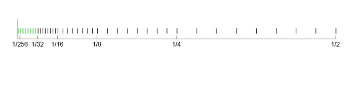
If you look carefully at the output from floatgui shown in the previous post you will see a gap around zero. This is especially apparent in the logarithmic plot, because the logarithmic distribution can never reach zero. Here is output for slightly different parameters, $t = 3$, $e_{min} = -5$, and $e_{max} = 2$. Howrever, the gap around zero has been filled in with a spot of green. Those are the denormals.
Zoom In
Zoom in on the portion of these toy floating point numbers less than one-half. Now you can see the individual green denormals -- there are eight of them in this case.
Denormal Floating Point Numbers
Denormal floating point numbers are essentially roundoff errors in normalized numbers near the underflow limit, realmin, which is $2^{-e_{max}+1}$. They are equally spaced, with a spacing of eps*realmin. Zero is naturally included as the smallest denormal. Suppose that x and y are two distinct floating point numbers near to, but larger than, realmin. It may well be that their difference, x - y, is smaller than realmin. For example, in the small floatgui system pictured above, eps = 1/8 and realmin = 1/32. The quantities x = 6/128 and y = 5/128 are between 1/32 and 1/16, so they are both above underflow. But x - y = 1/128 underflows to produce one of the green denormals. Before the IEEE standard, and even on today's systems that do not comply with the standard, underflows would simply be set to zero. So it would be possible to have the MATLAB expressionx == ybe false, while the expression
x - y == 0be true. On machines where underflow flushes to zero and division by zero is fatal, this code fragment can produce a division by zero and crash.
if x ~= y
   z = 1/(x-y);
end
Of course, denormals can also be produced by multiplications and divisions that produce a result between eps*realmin and realmin. In decimal these ranges are
   format compact
   format short e
   [eps*realmin realmin]
   [eps('single')*realmin('single') realmin('single')]
ans =
  4.9407e-324  2.2251e-308
ans =
  1.4013e-45  1.1755e-38
Denormal Format
Denormal floating point numbers are stored without the implicit leading one bit, $$ x = \pm f \cdot 2^{-emax+1}$$ The fraction $f$ satisfies $$ 0 \leq f < 1 $$ And $f$ is represented in binary using 52 bits for double precision and 23 bits for single recision. Note that zero naturally occurs as a denormal. When you look at a double precision denormal with format hex the situation is fairly clear. The rightmost 13 hex characters are the 52 bits of the fraction. The leading bit is the sign. The other 12 bits of the first three hex characters are all zero because they represent the biased exponent, which is zero because $emax$ and the exponent bias were chosen to complement each other. Here are the two largest and two smallest nonzero double precision denormals.format hex [(1-eps); (1-2*eps); 2*eps; eps; 0]*realmin format long e ans
ans =
   000fffffffffffff
   000ffffffffffffe
   0000000000000002
   0000000000000001
   0000000000000000
ans =
    2.225073858507201e-308
    2.225073858507200e-308
    9.881312916824931e-324
    4.940656458412465e-324
                         0
The situation is slightly more complicated with single precision because 23 is not a multiple of four. The fraction and exponent fields of a single precision floating point number -- normal or denormal -- share the bits in the third character of the hex display; the biased exponent gets one bit and the first three bits of the 23 bit fraction get the other three. Here are the two largest and two smallest nonzero single precision denormals.
   format hex
   e = eps('single');
   r = realmin('single');
   [(1-e); (1-2*e); 2*e; e; 0]*r
   format short e
   ans
ans =
   007fffff
   007ffffe
   00000002
   00000001
   00000000
ans =
  1.1755e-38
  1.1755e-38
  2.8026e-45
  1.4013e-45
           0
Think of the situation this way. The normalized floating point numbers immediately to the right of realmin, between realmin and 2*realmin, are equally spaced with a spacing of eps*realmin. If just as many numbers, with just the same spacing, are placed to the left of realmin, they fill in the gap between there and zero. These are the denormals. They require a slightly different format to represent and slightly different hardware to process.
IEEE Floating Point Committee
The IEEE Floating Point Committee was formed in 1977 in Silicon Valley. The participants included representatives of semiconductor manufacturers who were developing the chips that were to become the basis for the personal computers that are so familiar today. As I said in my previous post, the committee was a remarkable case of cooperation among competitors. Velvel Kahan was the most prominent figure in the committee meetings. He was not only a professor of math and computer science from UC Berkeley, he was also a consultant to Intel and involved in the design of their math coprocessor, the 8087. Some of Velvel's students, not only from the campus, but also who had graduated and were now working for some of the participating companies, were involved. A proposed standard, written by Kahan, one of his students at Berkeley, Jerome Coonen, and a visiting professor at Berkeley, Harold Stone, known as the KCS draft, reflected the Intel design and was the basis for much of the committee's work. The committee met frequently, usually in the evening in conference rooms of companies on the San Francisco peninsula. There were also meetings in Austin, Texas, and on the East Coast. The meetings often lasted until well after midnight. Membership was based on regular attendance. I was personally involved only when I was visiting Stanford, so I was not an official member. But I do remember telling a colleague from Sweden who was coming to the western United States for the first time that there were three sites that he had to be sure to see: the Grand Canyon, Las Vegas, and the IEEE Floating Point Committee.Controversy
The denormals in the KCS draft were something new to most of the committee. Velvel said he had experimented with them at the University of Toronto, but that was all. Standards efforts are intended to regularize existing practice, not introduce new designs. Besides, implementing denormals would reguire additional hardware, and additional transistors were a valuable resource in emerging designs. Some experts claimed that including denormals would slow down all floating point arithmetic. A mathematician from DEC, Mary Payne, led the opposition to KCS. DEC wanted a looser standard that would embrace the floating point that was already available on their VAX. The VAX format was similar to, but not the same as, the KCS proposal. And it did not include denormals. Discussion went on for a couple of years. Letters of support for KCS from Don Knuth and Jim Wilkinson did not settle the matter. Finally, DEC engaged G. W. (Pete) Stewart, from the University of Maryland. In what must have been a surprise to DEC, Pete also said he thought that the KCS proposal was a good idea. Eventually the entire committee voted to accept a revised version.Denormals Today
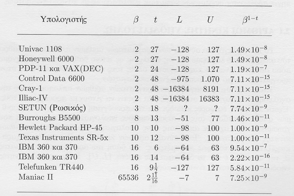
Denormal floating point numbers are still the unwanted step children in today's floating point family. I think it is fair to say that the numerical analysis community has failed to make a strong argument for their importance. It is true that they do make some floating point error analyses more elegant. But with magnitudes around $10^{-308}$ the double precision denormals are hardly ever numerically significant in actual computation. Only the single precision denormals around $10^{-38}$ are potentially important. Outside of MATLAB itself, we encounter processors that have IEEE format for the floating point numbers, but do not conform to the 754 standard when it comes to processing. These processors usually flush underflow to zero and so we can expect different numerical results for any calculations that might ordinarily produce denormals. We still see processors today that handle denormals with microcode or software. Execution time of MATLAB programs that encounter denormals can degrade significantly on such processors. The Wikipedia page on denormals has the macros for setting trap handlers to flush underflows to zero in C or Java programs. I hate to think what might happen to MATLAB Mex files with such macros. Kids, don't try this at home.References
William Kahan, Home Page. Charles Severance, An Interview with the Old Man of Floating-Point, Reminiscences for IEEE Computer, February 20, 1998. Wikipedia page, Denormal number. Published with MATLAB® R2014a

See Also
-

Floating Point Numbers
Blogs
-
-

コメント
コメントを残すには、ここ をクリックして MathWorks アカウントにサインインするか新しい MathWorks アカウントを作成します。