
Gaussian Elimination with Partial Pivoting
In rare cases, Gaussian elimination with partial pivoting is unstable. But the situations are so unlikely that we continue to use the algorithm as the foundation for our matrix computations.
Contents
Pivot Growth
I almost hesitate to bring this up. Gaussian elimination with partial pivoting is potentially unstable. We know of a particular test matrix, and have known about it for years, where the solution to simultaneous linear equations computed by our iconic backslash operator is less accurate than we typically expect. The solution is contaminated by unacceptably large roundoff errors associated with large elements encountered during the elimination process. The offending matrix is generated by the following function, which is a special case of the gfpp function in Nick Higham's collection of MATLAB test matrices.
type gfpp
function A = gfpp(n)
%  A = gfpp(n)  Pivot growth of partial pivoting.

   A = eye(n,n) - tril(ones(n,n),-1);
   A(:,n) = 1;
Here is the 8-by-8.
   n = 8
   A = gfpp(n)
n =
     8
A =
     1     0     0     0     0     0     0     1
    -1     1     0     0     0     0     0     1
    -1    -1     1     0     0     0     0     1
    -1    -1    -1     1     0     0     0     1
    -1    -1    -1    -1     1     0     0     1
    -1    -1    -1    -1    -1     1     0     1
    -1    -1    -1    -1    -1    -1     1     1
    -1    -1    -1    -1    -1    -1    -1     1
Gaussian elimination with partial pivoting does not actually do any pivoting with this particular matrix. The first row is added to each of the other rows to introduce zeroes in the first column. This produces twos in the last column. As similar steps are repeated to create an upper triangular U, elements in the last column double with each step. The element growth in the final triangular factor U is 2^(n-1).
   [L,U] = lu(A);
   U
U =
     1     0     0     0     0     0     0     1
     0     1     0     0     0     0     0     2
     0     0     1     0     0     0     0     4
     0     0     0     1     0     0     0     8
     0     0     0     0     1     0     0    16
     0     0     0     0     0     1     0    32
     0     0     0     0     0     0     1    64
     0     0     0     0     0     0     0   128
So if the matrix order n is set to the number of bits in the floating point word (plus one), the last diagonal element of U will grow to be 1/eps.
   n = 53
   A = gfpp(n);
   [L,U] = lu(A);
   unn = U(n,n)
n =
    53
unn =
   4.5036e+15
If we try to use backslash to solve a linear system involving this matrix and a random right hand side, the back substitution will begin with U(n,n). The roundoff errors can be expected to be as large as eps(U(n,n)) and swamp the solution itself.
   b = randn(n,1);
   x = A\b;
Ordinarily, we expect the solution computed by Gaussian elimination to have a residual on the order of roundoff error. But in this case, the residual is many orders of magnitude larger. Backslash has failed.
   r = b - A*x;
   relative_residual = norm(r)/(norm(A)*norm(x))
relative_residual =
   3.7579e-05
Swap Rows
Anything we do to this matrix to provoke pivoting during the elimination will prevent the growth of the elements in U. One possibility is to swap the first two rows.
   A = gfpp(n);
   A([1 2],:) = A([2 1],:);
   [L,U] = lu(A);
   unn = U(n,n)
unn =
     2
That's much better. Now use backslash and look at the residual.
   x = A\b;
   r = b - A*x;
   relative_residual = norm(r)/(norm(A)*norm(x))
relative_residual =
   1.7761e-17
So the residual is now on the order of roundoff relative to A and x. Backslash works as expected.
Introduce Noise
Another way to provoke pivoting is to perturb the matrix with a little white noise.
   A = gfpp(n);
   A = A + randn(n,n);
   [L,U] = lu(A);
   unn = U(n,n)
unn =
   -3.8699
So U is well behaved. Let's see about backslash.
   x = A\b;
   r = b - A*x;
   relative_residual = norm(r)/(norm(A)*norm(x))
relative_residual =
   1.2870e-16
Again the residual is on the order of roundoff and backslash works as expected.
Growth Factor
Suppose we are using Gaussian elimination with any pivoting process to solve a system of linear equations involving a matrix $A$. Let $a_{i,j}^{(k)}$ denote the elements in the matrix after the $k$ th step of the elimination. The growth factor for that pivoting process is the quantity
$$ \rho = { \max_{i,j,k} |a_{i,j}^{(k)}| \over \max_{i,j} |a_{i,j}| } $$
This growth factor is a crucial quantity in Wilkinson's roundoff error analysis. If $\rho$ is not too large, then the elimination algorithm is stable. Unfortunately, the matrix we have just seen, gfpp, shows that the growth factor for partial pivoting is at least $2^{n-1}$.
At the time he was presenting his analysis in early 1970s, Wilkinson knew about this matrix. But he said it was a very special case. He reported:
It is our experience that any substantial increase in size of elements of successive An is extremely uncommon even with partial pivoting. ... No example which has arisen naturally has in my experience given an increase as large as 16.
During the development of LINPACK in the late 1970s, a colleague at Argonne, J. T. Goodman, and I did some experiments with random matrices to check for element growth with partial pivoting. We used several different element distributions and what were then matrices of modest order, namely values of $n$ between 10 and 50. The largest growth factor we found was for a matrix of 0's and 1's of order 40. The value was $\rho$ = 23. We never saw growth as large as linear, $\rho = n$, let alone exponential, $\rho = 2^{n-1}$.
Average Case Growth
Nick Trefethen and Rob Schreiber published an important paper, "Average-case Stability of Gaussian Elimination", in 1990. They present both theoretical and probabilistic models, and the results of extensive experiments. They show that for many different types of matrices, the typical growth factor for partial pivoting does not increase exponentially with matrix order $n$. It does not even grow linearly. It actually grows like $n^{2/3}$. Their final section, "Conclusions", begins:
Is Gaussian elimination with partial pivoting stable on average? Everything we know on the subject indicates that the answer is emphatically yes, and that one needs no hypotheses beyond statistical properties to account for the success of this algorithm during nearly half a century of digital computation.
Worst Case Growth
The Higham Brothers, Nick and Des Higham, published a paper in 1989 about growth factors in Gaussian elimination. Most of their paper applies to any kind of pivoting and involves growth that is $O(n)$. But they do have one theorem that applies only to partial pivoting and that characterizes all matrices that have $\rho = 2^{n-1}$. Essentially these matrices have to have the behavior we have seen in gfpp, namely no actual pivoting and each step adds a row to all the later rows, doubling the values in the last column in the process.
Exponential Growth in Practice
In two different papers, Stephen Wright in 1993 and Les Foster in 1994, the authors present classes of matrices encountered in actual computational practice for which Gaussian elimination with partial pivoting blows up with exponential growth in the elements in the last few columns of U. Wright's application is a two-point boundary value problem for an ordinary differential equation. The discrete approximation produces a band matrix. Foster's application is a Volterra integral equation model for population dynamics. The discrete approximation produces a lower trapezoidal matrix. In both cases the matrices are augmented by several final columns. Certain choices of parameters causes the elimination to proceed with no pivoting and results in exponential in growth in the final columns. The behavior is similar to gfpp and the worst case growth in the Highams theorem.
Complete Pivoting
Complete pivoting requires $O(n^3)$ comparisons instead of the $O(n^2)$ required by partial pivoting. More importantly, the repeated access to the entire matrix complete changes the memory access patterns. With modern computer storage hierarchy, including cache and virtual memory, this is an all-important consideration.
The growth factor $\rho$ with complete pivoting is interesting and I plan to investigate it in my next blog.
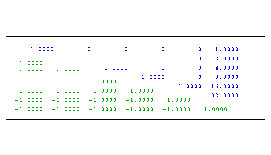
lugui
lugui is one of the demonstration programs included with Numerical Computing with MATLAB. I will also describe it in my next blog. For now, I will just use it to generate a graphic for this blog. Here is the result of a factorization, the lower triangular factor L in green and the upper triangular factor U in blue.
   A = gfpp(6);
   lugui(A,'partial')
References
Nicholas J. Higham and Desmond J. Higham, "Large Growth Factors in Gaussian Elimination with Pivoting", <http://www.maths.manchester.ac.uk/~higham/papers/hihi89.pdf>, SIAM J. Matrix Anal. Appl. 10, 155-164, 1989.
Lloyd N. Trefethen and Robert S. Schreiber, "Average-case Stability of Gaussian Elimination", SIAM J. Matrix Anal. Appl. 11, 335-360, 1990.
Stephen J. Wright, A Collection of Problems for Which Gaussian "Elimination with Partial Pivoting is Unstable", <ftp://info.mcs.anl.gov/pub/tech_reports/reports/P266.ps.Z>, SIAM J. Sci. Statist. Comput. 14, 231-238, 1993.
Leslie Foster, "Gaussian Elimination Can Fail In Practice", <http://www.math.sjsu.edu/~foster/geppfail.pdf>, SIAM J. Matrix Anal. Appl. 15, 1354-1362, 1994.
- Category:
- History,
- Matrices,
- Numerical Analysis


Comments
To leave a comment, please click here to sign in to your MathWorks Account or create a new one.