 Cleve’s Corner: Cleve Moler on Mathematics and Computing
 The MATLAB Blog
 Guy on Simulink
 MATLAB Community
 Artificial Intelligence
 Developer Zone
 Stuart’s MATLAB Videos
 Behind the Headlines
 File Exchange Pick of the Week
 Hans on IoT
 Student Lounge
 MATLAB ユーザーコミュニティー
 Startups, Accelerators, & Entrepreneurs
 Autonomous Systems
 Quantitative Finance
 MATLAB Graphics and App Building
Modernization of Numerical Integration, From Quad to Integral
The MATLAB functions for the numerical evaluation of integrals has evolved from quad, through quadl and quadgk, to today's integral.

 The algorithm works recursively on subintervals of the original interval [a,b]. If the values obtained from the 3-point Simpson's rule and the 5-point composite Simpson's rule agree to within a specified tolerance (which they clearly do not for these figures), then an extrapolation taken from the two values is accepted as the value for the integral over the subinterval. If not, the algorithm is recursively applied to the two halves of the subinterval.
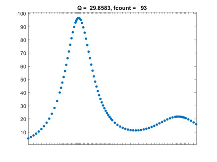
 Here is the final result. The default tolerance for quad is $10^{-6}$ and the value of the integral obtained to six significant digits is 29.8583. The integrand has been evaluated 93 times. Most of those evaluations took place near the peaks where the humps varies rapidly. This indicates that the adaptivity works as expected.
 Humps is a rational function. It is possible to use the Symbolic Toolbox to obtain the indefinite and then the definite integral analytically.
Contents
Quadrature
Several years ago I regarded myself as an expert on numerical methods for approximating integrals. But then I stopped paying attention for a while. So this is an opportunity to get reacquainted. The task involves a real-valued function $f(x)$ of a real variable $x$, defined on an interval $a \le x \le b$. We seek to compute the value of the definite integral, $$ \int_a^b \ f(x) \ dx $$ I wrote a chapter on the subject in my textbook Numerical Computing with MATLAB. Here is a link to that chapter. The chapter is titled "Quadrature". One of the first things I have to do in that chapter is explain that quadrature is an old-fashioned term derived from the notion that the value of a definite integral can be approximated by plotting the function on graph paper and then counting the number of little squares that fall underneath the graph. Here is a coarse picture.
Adaptive Simpson's method and quad
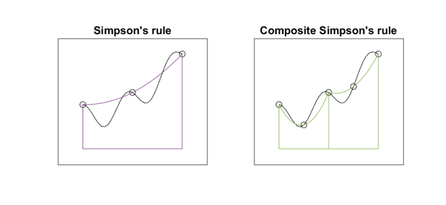
For most of the time since the beginning of MATLAB, up until when I wrote the chapter on quadrature twelve years ago, the MATLAB function for evaluating definite integrals was one named quad. It was based on adaptive Simpson's method, pioneered by my grad school buddy Bill McKeeman to show off recursion in Algol. These two figures illustrate the basis for adaptive Simpson's method.
The algorithm works recursively on subintervals of the original interval [a,b]. If the values obtained from the 3-point Simpson's rule and the 5-point composite Simpson's rule agree to within a specified tolerance (which they clearly do not for these figures), then an extrapolation taken from the two values is accepted as the value for the integral over the subinterval. If not, the algorithm is recursively applied to the two halves of the subinterval.
Humps and quadgui
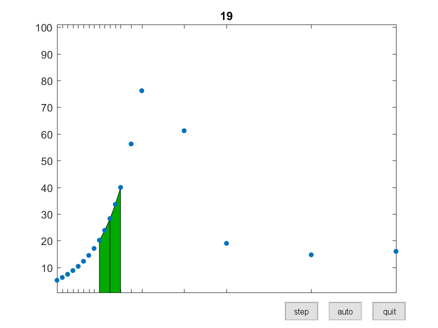
I have used a function named humps to demonstrate numerical integration for a long time. It has a strong peak at x = 0.3 and a milder peak at x = 0.9. It has found its way into the MATLAB demos directory, so you have it on your own machine. A graph appears below. $$ h(x) = \frac{1}{(x-0.3)^2+.01} + \frac{1}{(x-0.9)^2+.04} - 6 $$ An interactive graphical app named quadgui is included with the programs for Numerical Computing with MATLAB, available from MATLAB Central File Exchange. It shows quad in action. Here is a snapshot of quad part way through computing the integral of humps over the interval [0,1]. Integration over the interval to the left of 1/4 is finished. The integration over the subinterval [1/4,3/8] has just been successfully completed. A few samples to the right of 3/8 were computed during the initialization. The integrand has been evaluated 19 times.
Here is the final result. The default tolerance for quad is $10^{-6}$ and the value of the integral obtained to six significant digits is 29.8583. The integrand has been evaluated 93 times. Most of those evaluations took place near the peaks where the humps varies rapidly. This indicates that the adaptivity works as expected.
Humps is a rational function. It is possible to use the Symbolic Toolbox to obtain the indefinite and then the definite integral analytically.
   syms x
   h = 1/((x-3/10)^2+1/100) + 1/((x-9/10)^2+4/100) - 6
   I = int(h,x)
   D = subs(I,1)-subs(I,0)
   format long
   Q = double(D)
h =
1/((x - 9/10)^2 + 1/25) + 1/((x - 3/10)^2 + 1/100) - 6
I =
10*atan(10*x - 3) - 6*x + 5*atan(5*x - 9/2)
D =
5*atan(1/2) + 10*atan(3) + 10*atan(7) + 5*atan(9/2) - 6
Q =
  29.858325395498674
This confirms the six figure value shown by quadqui


评论
要发表评论,请点击 此处 登录到您的 MathWorks 帐户或创建一个新帐户。