Lake Arrowhead Coauthor Graph Revisited
The Lake Arrowhead Coauthor Graph came out of the Householder XII conference in 1993 at the UCLA conference center in the mountains north of San Bernardino. John Gilbert now remembers it as one of the first computational social network analyses he had ever seen. Today I revisit it using the new MATLAB graph object.
Contents
Coauthor Graph
I wrote a blog post about the Lake Arrowhead Coauthor Graph a couple of years ago.
At the Householder XII conference in 1993 Nick Trefethen posted a flip chart with Gene Golub's name in the center. He invited everyone present to add their name to the chart and draw lines connecting their name with the names of all their coauthors. The diagram grew denser throughout the week. At the end of the conference it was a graph with 104 vertices (or people) and 211 edges.
Nick framed the original chart and has it on the wall of his office at Oxford. Another Nick, Nick Hale, took this photo.

The Data
John Gilbert, Rob Schreiber and I entered the names and coauthor connections into MATLAB, creating an adjacency matrix A. For a long time the data was available as a .mat file from John's old web site at Xerox PARC. But John left PARC years ago, so I am now making the data available in human-readable form at the end of this blog post. There are two files.
   A = arrowhead_adjacency;
   names = arrowhead_names;
Reverse Cuthill-McGee
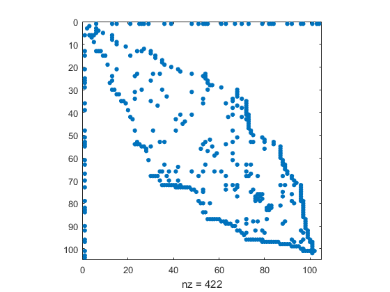
The ordering of the authors in the original data is determined by how we happened to read them off the flip chart. Golub is first, and has the most connections to other authors. A symmetric reverse Cuthill-McGee ordering of the rest of the nodes puts coauthors near each other and reduces the band width of the adjacency matrix.
   r = [1 symrcm(A(2:end,2:end))+1];
   A = A(r,r);
   names = names(r);
   spy(A)
Circle Layout
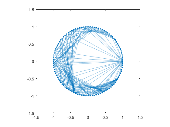
Let's make a MATLAB graph and plot it with the circle layout. By default, the graph/plot method omits the node names if there are more than 100 of them. This removes clutter and is usually a good idea. The resulting unannotated circle layout is a pretty picture, but not very informative.
The RCM ordering places most of the graph edges, except those connecting to Golub, near the circumference of the circle.
   G = graph(A,names);
   plot(G,'layout','circle')
   axis square
Node Names
Move Golub to the center.
   p = plot(G,'Layout','circle');
   idGolub = findnode(G,'Golub');
   p.XData(idGolub) = 0;
   p.YData(idGolub) = 0;
   axis square

Placing the rest of the names around the outside of the circle requires some custom processing.
   axis off
   t = text(p.XData,p.YData,names);
   theta = linspace(0,360,numel(t)+1);
   for k = 1:numel(t)
       t(k).Rotation = theta(k);
       t(k).String = [blanks(4) t(k).String];
       t(k).FontSize = 8;
   end

This plot can now be compared with the plot we originally produced at Householder XII.
Three-Dimensional Layout
In this two-dimensional circle plot it's nearly impossible to follow the links from one author to his or her coauthors. 'Moler' is at about 5 o'clock on the circle. What is the degree of my node? Who are my coauthors?
A three-dimensional layout and judicious use of the mouse in conjunction with cameratoolbar makes it possible to examine this graph in detail.
   p = plot(G,'layout','force3','nodelabelmode','auto');
   % Setting the nodelabelmode says include all of the names.
   axis off vis3d
   set(gca,'clipping','off')
   zoom(2)
   gif_frame('arrowhead_name.gif')
   gif_frame(2)

Moler's Coauthors
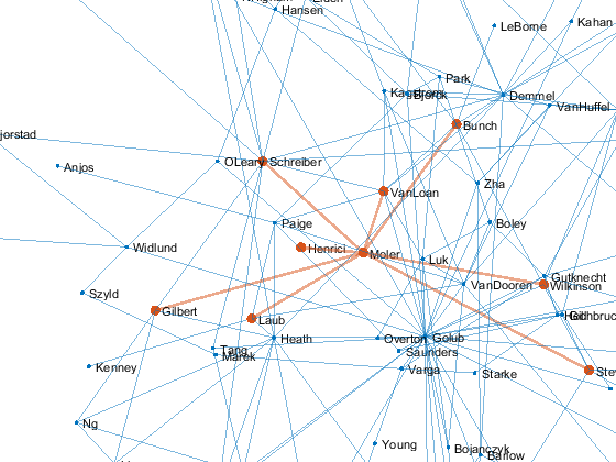
Let's highlight me and my coauthors.
   me = findnode(G,'Moler')
   friends = neighbors(G,me)'
   color = get(gca,'colororder');
   highlight(p,[me friends],'nodecolor',color(2,:),'markersize',6)
   highlight(p,me,friends,'edgecolor',color(2,:),'linewidth',2)
   gif_frame(2)
me =
    88
friends =
    61    62    63    68    75    77    89    98

Center
Make my node the center of this little universe.
   set(p,'xdata',p.XData - p.XData(me), ...
         'ydata',p.YData - p.YData(me), ...
         'zdata',p.ZData - p.ZData(me))
   gif_frame(2)
Zoom
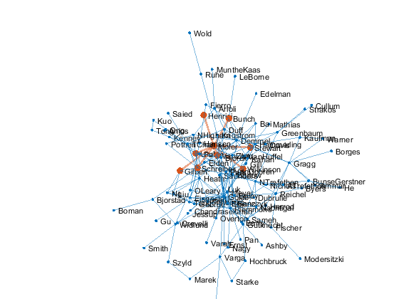
Now zoom and rotate. This is much better done in person with cameratoolbar. The best we can do in this blog is an animated gif.
   % Zoom
   for k = 1:4
       zoom(sqrt(2))
       gif_frame
   end

   % Rotate
   [a,e] = view;
   for k = 1:4
       view(a,e-12*k)
       gif_frame
   end
   gif_frame(5)
Animation
Here is the animated .gif centered on me and my coauthors.
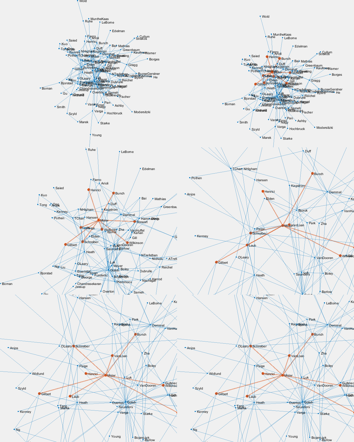
And here we zoom in on Paul VanDooren by replacing
me = findnode(G,'Moler')
with
me = findnode(G,'VanDooren')

arrowhead_adjacency.m
   function A = arrowhead_adjacency
     k = [ 1  1   1   1   1   3   3   1   1   1   1   2   3   3  38   1   2 ...
     32  42   3  32  42  43  44  44   1  46   1   1  37  13  49   1  32   1 ...
     44  53   1  53  44  45  54   1   1  20  41  44   1  39  52  60  15  58 ...
     61   3  63  41  43   1  15  35  51  61  41  43  59  65  53   3  58  63 ...
     42   1  41  44   1  46  47   1  10  15  32  35  62  66   2  19  39  58 ...
     61  66  69  37  53   1   9  72  42   8  21  32  42  77   1   7  15  46 ...
     47  49   6  42  66   1   3  25  41  43  59  65  67  80  33  52  59  27 ...
     28  46  74  31  51  46   1  22  23  24  25  35  41  52  81   3  21  55 ...
     60  44  58  62   4  17  12  19  23  72  77  89   1  23  86   1  23  86 ...
     91   4  72  90  19  90  48   1  18  25  77  82  86  17  52  66  86  89 ...
     16  32  34  58  66  80  81   1  34  74  77  14  82  77  79  49 102  26 ...
     32  39  44  48  51  52  56  63  69  74  78  81  83  90];

     j = [ 2  3   5  10  11  29  30  32  34  35  36  36  38  40  40  41  42 ...
     42  43  44  44  44  44  45  46  47  47  48  49  49  50  50  51  51  53 ...
     54  54  55  55  56  56  57  58  59  59  59  59  60  60  60  61  62  62 ...
     62  63  64  65  65  66  66  66  66  66  67  67  67  67  68  69  69  69 ...
     70  71  71  71  72  72  72  73  73  73  73  73  73  73  74  74  74  74 ...
     74  74  74  75  75  76  76  76  77  78  78  78  78  78  79  79  79  79 ...
     79  79  80  80  80  81  81  81  81  81  81  81  81  81  82  82  82  83 ...
     83  83  83  84  84  85  86  86  86  86  86  86  86  86  86  87  87  87 ...
     87  88  88  88  89  89  90  90  90  90  90  90  91  91  91  92  92  92 ...
     92  93  93  93  94  94  95  96  96  96  96  96  96  97  97  97  97  97 ...
     98  98  98  98  98  98  98  99  99  99  99 100 100 101 102 103 103 104 ...
     104 104 104 104 104 104 104 104 104 104 104 104 104 104];

     U = sparse(k,j,1,104,104);
     A = logical(U + U');
  end
arrowhead_names.m
  function names = arrowhead_names
    names = {'Golub', 'Wilkinson', 'TChan', 'He', 'Varah', 'Kenney', ...
    'Ashby', 'LeBorne', 'Modersitzki', 'Overton', 'Ernst', 'Borges', ...
    'Kincaid', 'Crevelli', 'Boley', 'Anjos', 'Byers', 'Benzi', 'Kaufman', ...
    'Gu', 'Fierro', 'Nagy', 'Harrod', 'Pan', 'Funderlic', 'Edelman', ...
    'Cullum', 'Strakos', 'Saied', 'Ong', 'Wold', 'VanLoan', ...
    'Chandrasekaran', 'Saunders', 'Bojanczyk', 'Dubrulle', 'Marek', ...
    'Kuo', 'Bai', 'Tong', 'George', 'Moler', 'Gilbert', 'Schreiber', ...
    'Pothen', 'NTrefethen', 'Nachtigal', 'Kahan', 'Varga', 'Young', ...
    'Kagstrom', 'Barlow', 'Widlund', 'Bjorstad', 'OLeary', 'NHigham', ...
    'Boman', 'Bjorck', 'Eisenstat', 'Zha', 'VanHuffel', 'Park', 'Arioli', ...
    'MuntheKaas', 'Ng', 'VanDooren', 'Liu', 'Smith', 'Duff', 'Henrici', ...
    'Tang', 'Reichel', 'Luk', 'Hammarling', 'Szyld', 'Fischer', ...
    'Stewart', 'Bunch', 'Gutknecht', 'Laub', 'Heath', 'Ipsen', ...
    'Greenbaum', 'Ruhe', 'ATrefethen', 'Plemmons', 'Hansen', 'Elden', ...
    'BunseGerstner', 'Gragg', 'Berry', 'Sameh', 'Ammar', 'Warner', ...
    'Davis', 'Meyer', 'Nichols', 'Paige', 'Gill', 'Jessup', 'Mathias', ...
    'Hochbruck', 'Starke', 'Demmel'};
  end
Thanks
Special thanks to Christine Tobler and Cosmin Ionita at MathWorks for help with today's post.
- Category:
- Graphics


Comments
To leave a comment, please click here to sign in to your MathWorks Account or create a new one.