I am addicted. I keep coming back to John Conway's Game of Life. Years ago, I wrote a chapter about Life in Experiments with MATLAB. I wrote a three-part series about Life shortly after I started blogging. Part 1, Part 2, Part 3. I have recently made significant enhancements to my MATLAB program for Life. I never seem to finish the code because I get diverted by actually using the program to explore the Universe. I invite you to join me. But, fair warning, you might become addicted too.

Contents

The Rule

Recall how the Game of Life works. The universe is an infinite, two-dimensional rectangular grid. The population is a collection of grid cells that are marked as alive. The population evolves at discrete time steps known as generations. At each step, the fate of each cell is determined by the vitality of its eight nearest neighbors and this rule:

The fascination of Life is that this deceptively simple rule leads to an incredible variety of patterns, puzzles, and unsolved problems.

Code

Here is the core of the code. Sparse indexing makes it look easy. The graphics is done by the sparse display program, spy.

   dbtype 69:85 life_lex

69              % Whether cells stay alive, die, or generate new cells depends
70              % upon how many of their eight possible neighbors are alive.
71              % Index vectors increase or decrease the centered index by one.
72    
73              n = size(X,1);
74              p = [1 1:n-1];
75              q = [2:n n];
76    
77              % Count how many of the eight neighbors are alive.
78    
79              Y = X(:,p) + X(:,q) + X(p,:) + X(q,:) + ...
80                  X(p,p) + X(q,q) + X(p,q) + X(q,p);
81    
82              % A live cell with two live neighbors, or any cell with
83              % three live neigbhors, is alive at the next step.
84    
85              X = (X & (Y == 2)) | (Y == 3);

Infinite Universe

So how, exactly, does an infinite universe work? The same question is asked by astrophysicists and cosmologists about our own universe. Over the years, I have offered several MATLAB Game of Life programs that have tackled this question in different ways. I finally have a solution that I like.

In all my programs, the population is represented by a sparse matrix. This means that the storage requirement, and the execution time, are proportional to the size of the population, not to the size of some grid. The sparse matrix readily accommodates a growing population. There are no boundaries and consequently no boundary conditions.

But how do I display an infinite universe? In the past I've had a window that is a snapshot of the entire population. But many interesting Life configurations throw off isolated gliders. These are five-celled objects that move forever in one direction. (Think of Voyager I.) A display window that includes all of the gliders must expand accordingly. This means the rest of the population, which often remains bounded, is relegated to a shrinking fraction of the window. The solution is to let isolated gliders leave the display window and count them as they go.

Glider

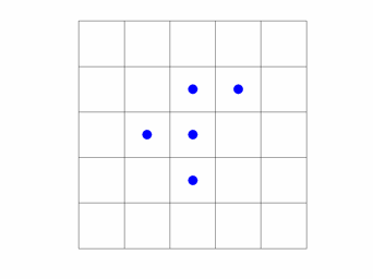
My first example is a single glider. At each step two cells die, and two new ones are born. After four steps the original population reappears, but it has moved diagonally up and across the grid. It moves in this direction forever, continuing to exist in the infinite universe. This animated gif shows every step for the first eight steps, then captures every fourth step. When the glider reaches the edge of the window, it is counted and disappears from view. The clock continues to run, even though there is nothing to see.

Life Lexicon

My latest program is called life_lex. The starting populations for life_lex are obtained from the Life Lexicon, a valuable Web resource cataloging well over a thousand terms related to the Game of Life. The Lexicon now includes almost seven hundred starting populations. The supporting community is very active -- many discoveries have been made in the last few years. You can see the entire collection by selecting "slide show" in the life_lex menu. The show lasts about 11 minutes.

The Lexicon is available in two forms. The text form is used by life_lex and is distributed with it as lexicon.txt. The HTML form, which is extensively cross linked, is available on the Web. The lexicon toggle provides the link.

Herschel

Named after the guy who discovered Uranus in 1781. As to how it came to be named after him, you will have to read the Lexicon. It is one of the most frequent features occurring in larger populations. It starts with a heptomino, a population of size 7. The population grows to over 100 before it reaches a steady state of size 24 at time 128. It creates two gliders in the process.

Here are the first eight generations and every fourth one after that.

Fx77

The story behind the name of this configuration is very technical. "Fx" means the signal moves forward and produces a mirror-image output. The "77" comes from the fact that a pair of Herschels appear at time 77. Notice that if you cut the window in half horizontally, the two halves have very similar subpopulations. The population count begins at 67 at time zero, reaches a maximum of 294 at time 179, and eventually stabilizes at 104 for time greater than 206.

Fx77 creates seven gliders. I've been using it to test my glider counting code. It is a good example of a population that remains bounded in space except for its gliders. Here is every tenth generation.

Soup

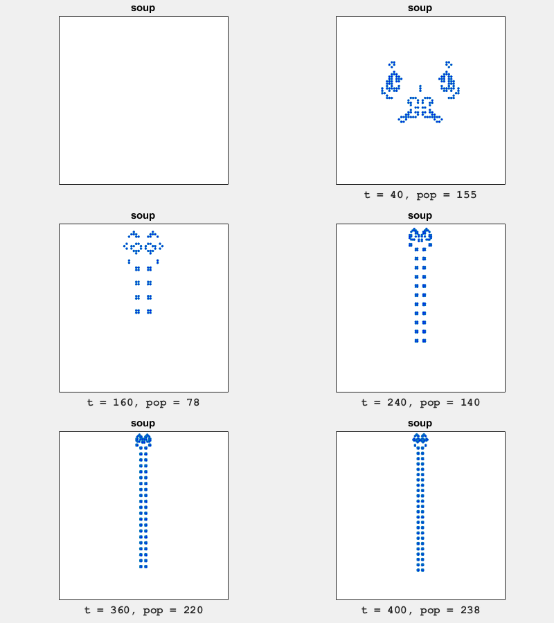
There are many flavors of soup. This example is a massive population that is unbounded and does not produce any gliders. The Lexicon informs us that it is an unusual mirror-symmetric soup that produces a pufferfish and nothing else.

life_lex

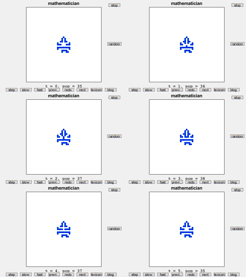
Here is a screen shot of my latest program, life_lex. The toggles let you select the display time for a generation -- single step, slow, or fast. You can page forward or backward through the Lexicon. You can access this blog post. You can select from a menu of more than a dozen suggestions, populations that I have found especially interesting.

Here is the current list in the suggestions menu. It's subject to change as I come across other goodies.

         'random'
         'pre-block'
         'blinker'
         'glider'
         'Gosper glider gun'
         'Gabriel''s p138'
         'Snark'
         'spacefiller'
         'Fx77'
         'against the grain'
         'soup'
         'block and glider'
         'lightspeed'
         'volatility'
         'gliders by the dozen'
         'total aperiodic' ....
         'Noah''s ark'
         'slide show'

I will include life_lex in a new release, 3.8, of Cleve's Laboratory.

In case you want life_lex by itself, I will submit it separately to https://www.mathworks.com/matlabcentral/fileexchange/69383-game-of-life. The submission includes a copy of Lexicon.txt.

Get the MATLAB code

Published with MATLAB® R2018a