
Semantic Segmentation Using Deep Learning
Today I want to show you a documentation example that shows how to train a semantic segmentation network using deep learning and the Computer Vision System Toolbox.
A semantic segmentation network classifies every pixel in an image, resulting in an image that is segmented by class. Applications for semantic segmentation include road segmentation for autonomous driving and cancer cell segmentation for medical diagnosis. To learn more, see Semantic Segmentation Basics.
To illustrate the training procedure, this example trains SegNet, one type of convolutional neural network (CNN) designed for semantic image segmentation. Other types networks for semantic segmentation include fully convolutional networks (FCN) and U-Net. The training procedure shown here can be applied to those networks too.
This example uses the CamVid dataset from the University of Cambridge for training. This dataset is a collection of images containing street-level views obtained while driving. The dataset provides pixel-level labels for 32 semantic classes including car, pedestrian, and road.
Setup
This example creates the SegNet network with weights initialized from the VGG-16 network. To get VGG-16, install Neural Network Toolbox™ Model for VGG-16 Network. After installation is complete, run the following code to verify that the installation is correct.
vgg16();
In addition, download a pretrained version of SegNet. The pretrained model allows you to run the entire example without having to wait for training to complete.
pretrainedURL = 'https://www.mathworks.com/supportfiles/vision/data/segnetVGG16CamVid.mat';
pretrainedFolder = fullfile(tempdir,'pretrainedSegNet');
pretrainedSegNet = fullfile(pretrainedFolder,'segnetVGG16CamVid.mat');
if ~exist(pretrainedFolder,'dir')
    mkdir(pretrainedFolder);
    disp('Downloading pretrained SegNet (107 MB)...');
    websave(pretrainedSegNet,pretrainedURL);
end
Downloading pretrained SegNet (107 MB)...
A CUDA-capable NVIDIA™ GPU with compute capability 3.0 or higher is highly recommended for running this example. Use of a GPU requires Parallel Computing Toolbox™.
Download CamVid Dataset
Download the CamVid dataset from the following URLs.
imageURL = 'http://web4.cs.ucl.ac.uk/staff/g.brostow/MotionSegRecData/files/701_StillsRaw_full.zip';
labelURL = 'http://web4.cs.ucl.ac.uk/staff/g.brostow/MotionSegRecData/data/LabeledApproved_full.zip';
outputFolder = fullfile(tempdir,'CamVid');
if ~exist(outputFolder, 'dir')

    mkdir(outputFolder)
    labelsZip = fullfile(outputFolder,'labels.zip');
    imagesZip = fullfile(outputFolder,'images.zip');

    disp('Downloading 16 MB CamVid dataset labels...');
    websave(labelsZip, labelURL);
    unzip(labelsZip, fullfile(outputFolder,'labels'));

    disp('Downloading 557 MB CamVid dataset images...');
    websave(imagesZip, imageURL);
    unzip(imagesZip, fullfile(outputFolder,'images'));
end
Note: Download time of the data depends on your Internet connection. The commands used above block MATLAB until the download is complete. Alternatively, you can use your web browser to first download the dataset to your local disk. To use the file you downloaded from the web, change the
Load CamVid Images
Use imageDatastore to load CamVid images. The
imgDir = fullfile(outputFolder,'images','701_StillsRaw_full');
imds = imageDatastore(imgDir);
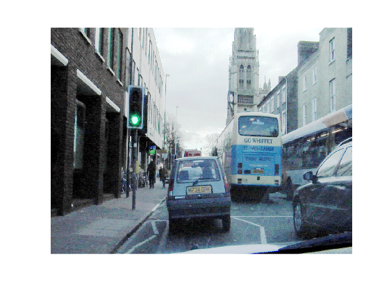
Display one of the images.
I = readimage(imds,1);
I = histeq(I);
imshow(I)
Load CamVid Pixel-Labeled Images
Use imageDatastore to load CamVid pixel label image data. A
Following the procedure used in original SegNet paper (Badrinarayanan, Vijay, Alex Kendall, and Roberto Cipolla. "SegNet: A Deep Convolutional Encoder-Decoder Architecture for Image Segmentation." arXiv preprint arXiv:1511.00561, 201), group the 32 original classes in CamVid to 11 classes. Specify these classes.
classes = [
    "Sky"
    "Building"
    "Pole"
    "Road"
    "Pavement"
    "Tree"
    "SignSymbol"
    "Fence"
    "Car"
    "Pedestrian"
    "Bicyclist"
    ];
To reduce 32 classes into 11, multiple classes from the original dataset are grouped together. For example, "Car" is a combination of "Car", "SUVPickupTruck", "Truck_Bus", "Train", and "OtherMoving". Return the grouped label IDs by using the supporting function
labelIDs = camvidPixelLabelIDs();
Use the classes and label IDs to create the
labelDir = fullfile(outputFolder,'labels');
pxds = pixelLabelDatastore(labelDir,classes,labelIDs);
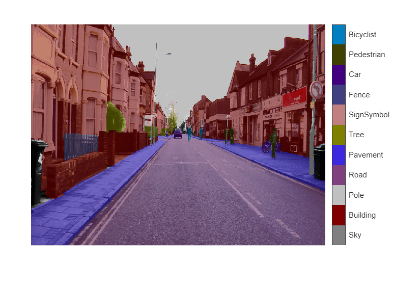
Read and display one of the pixel-labeled images by overlaying it on top of an image.
C = readimage(pxds,1);
cmap = camvidColorMap;
B = labeloverlay(I,C,'ColorMap',cmap);
imshow(B)
pixelLabelColorbar(cmap,classes);
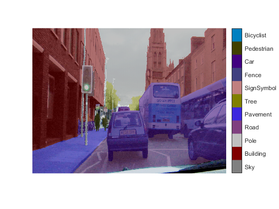
Areas with no color overlay do not have pixel labels and are not used during training.
Analyze Dataset Statistics
To see the distribution of class labels in the CamVid dataset, use countEachLabel. This function counts the number of pixels by class label.
tbl = countEachLabel(pxds)
tbl=11×3 table
        Name        PixelCount    ImagePixelCount
    ____________    __________    _______________
    'Sky'            76801167        483148800
    'Building'      117373718        483148800
    'Pole'            4798742        483148800
    'Road'          140535728        484531200
    'Pavement'       33614414        472089600
    'Tree'           54258673        447897600
    'SignSymbol'      5224247        468633600
    'Fence'           6921061        251596800
    'Car'            24436957        483148800
    'Pedestrian'      3402909        444441600
    'Bicyclist'       2591222        261964800
Visualize the pixel counts by class.
frequency = tbl.PixelCount/sum(tbl.PixelCount);
bar(1:numel(classes),frequency)
xticks(1:numel(classes))
xticklabels(tbl.Name)
xtickangle(45)
ylabel('Frequency')
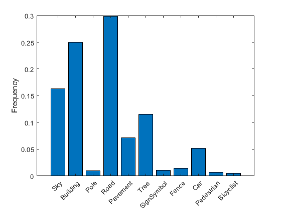
Ideally, all classes would have an equal number of observations. However, the classes in CamVid are imbalanced, which is a common issue in automotive datasets of street scenes. Such scenes have more sky, building, and road pixels than pedestrian and bicyclist pixels because sky, buildings and roads cover more area in the image. If not handled correctly, this imbalance can be detrimental to the learning process because the learning is biased in favor of the dominant classes. Later on in this example, you will use class weighting to handle this issue.
Resize CamVid Data
The images in the CamVid data set are 720 by 960. To reduce training time and memory usage, resize the images and pixel label images to 360 by 480.
imageFolder = fullfile(outputFolder,'imagesResized',filesep);
imds = resizeCamVidImages(imds,imageFolder);
labelFolder = fullfile(outputFolder,'labelsResized',filesep);
pxds = resizeCamVidPixelLabels(pxds,labelFolder);
Prepare Training and Test Sets
SegNet is trained using 60% of the images from the dataset. The rest of the images are used for testing. The following code randomly splits the image and pixel label data into a training and test set.
[imdsTrain,imdsTest,pxdsTrain,pxdsTest] = partitionCamVidData(imds,pxds);
The 60/40 split results in the following number of training and test images:
numTrainingImages = numel(imdsTrain.Files)
numTrainingImages =
   421
numTestingImages = numel(imdsTest.Files)
numTestingImages =
   280
Create the Network
Use segnetLayers to create a SegNet network initialized using VGG-16 weights.
imageSize = [360 480 3];
numClasses = numel(classes);
lgraph = segnetLayers(imageSize,numClasses,'vgg16');
The image size is selected based on the size of the images in the dataset. The number of classes is selected based on the classes in CamVid.
Balance Classes Using Class Weighting
As shown earlier, the classes in CamVid are not balanced. To improve training, you can use class weighting to balance the classes. Use the pixel label counts computed earlier with countEachLayer and calculate the median frequency class weights.
imageFreq = tbl.PixelCount ./ tbl.ImagePixelCount;
classWeights = median(imageFreq) ./ imageFreq
classWeights = 11×1

   0.318184709354742
   0.208197860785155
   5.092367332938507
   0.174381825257403
   0.710338097812948
   0.417518560687874
   4.537074815482926
   1.838648261914560
   1.000000000000000
   6.605878573155874
      ⋮
Specify the class weights using a pixelClassificationLayer.
pxLayer = pixelClassificationLayer('Name','labels','ClassNames',tbl.Name,'ClassWeights',classWeights)
pxLayer =
  PixelClassificationLayer with properties:

            Name: 'labels'
      ClassNames: {11×1 cell}
    ClassWeights: [11×1 double]
      OutputSize: 'auto'
   Hyperparameters
    LossFunction: 'crossentropyex'
Update the SegNet network with the new
lgraph = removeLayers(lgraph,'pixelLabels');
lgraph = addLayers(lgraph, pxLayer);
lgraph = connectLayers(lgraph,'softmax','labels');
Select Training Options
The optimization algorithm used for training is stochastic gradient descent with momentum (SGDM). Use trainingOptions to specify the hyperparameters used for SGDM.
options = trainingOptions('sgdm', ...
    'Momentum',0.9, ...
    'InitialLearnRate',1e-3, ...
    'L2Regularization',0.0005, ...
    'MaxEpochs',100, ...
    'MiniBatchSize',4, ...
    'Shuffle','every-epoch', ...
    'VerboseFrequency',2);
A minibatch size of 4 is used to reduce memory usage while training. You can increase or decrease this value based on the amount of GPU memory you have on your system.
Data Augmentation
Data augmentation is used during training to provide more examples to the network because it helps improve the accuracy of the network. Here, random left/right reflection and random X/Y translation of +/- 10 pixels is used for data augmentation.
augmenter = imageDataAugmenter('RandXReflection',true,...
    'RandXTranslation',[-10 10],'RandYTranslation',[-10 10]);
Start Training
Combine the training data and data augmentation selections using pixelLabelImageDatastore. The
pximds = pixelLabelImageDatastore(imdsTrain,pxdsTrain,...
    'DataAugmentation',augmenter);
Start training if the
doTraining = false;
if doTraining
    [net, info] = trainNetwork(pximds,lgraph,options);
else
    data = load(pretrainedSegNet);
    net = data.net;
end
Test Network on One Image
As a quick sanity check, run the trained network on one test image.
I = read(imdsTest);
C = semanticseg(I, net);
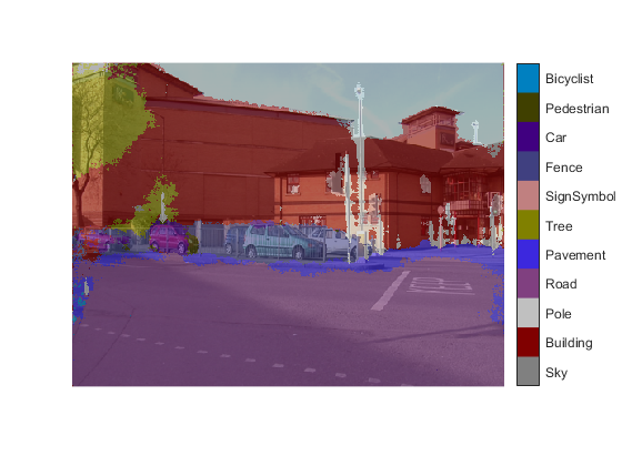
Display the results.
B = labeloverlay(I,C,'Colormap',cmap,'Transparency',0.4);
imshow(B)
pixelLabelColorbar(cmap, classes);
Compare the results in
expectedResult = read(pxdsTest);
actual = uint8(C);
expected = uint8(expectedResult);
imshowpair(actual, expected)
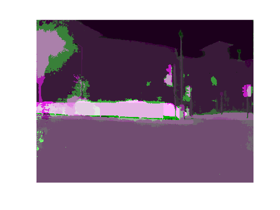
Visually, the semantic segmentation results overlap well for classes such as road, sky, and building. However, smaller objects like pedestrians and cars are not as accurate. The amount of overlap per class can be measured using the intersection-over-union (IoU) metric, also known as the Jaccard index. Use the jaccard function to measure IoU.
iou = jaccard(C, expectedResult);
table(classes,iou)
ans=11×2 table
      classes              iou
    ____________    __________________
    "Sky"            0.926585343977038
    "Building"       0.798698991022729
    "Pole"           0.169776501947919
    "Road"           0.951766120547122
    "Pavement"       0.418766821629557
    "Tree"           0.434014251781473
    "SignSymbol"     0.325092056812204
    "Fence"           0.49200469780468
    "Car"           0.0687557042896258
    "Pedestrian"                     0
    "Bicyclist"                      0
The IoU metric confirms the visual results. Road, sky, and building classes have high IoU scores, while classes such as pedestrian and car have low scores. Other common segmentation metrics include the Dice index and the Boundary-F1 contour matching score.
Evaluate Trained Network
To measure accuracy for multiple test images, run semanticseg on the entire test set.
pxdsResults = semanticseg(imdsTest,net,'MiniBatchSize',4,'WriteLocation',tempdir,'Verbose',false);
metrics = evaluateSemanticSegmentation(pxdsResults,pxdsTest,'Verbose',false);
metrics.DataSetMetrics
ans=1×5 table
     GlobalAccuracy        MeanAccuracy            MeanIoU            WeightedIoU         MeanBFScore
    _________________    _________________    _________________    _________________    ________________
    0.882035049405331    0.850970241394654    0.608927281006314    0.797947090677593    0.60980715338674
The dataset metrics provide a high-level overview of the network performance. To see the impact each class has on the overall performance, inspect the per-class metrics using
metrics.ClassMetrics
ans=11×3 table
                      Accuracy                IoU              MeanBFScore
                  _________________    _________________    _________________
    Sky           0.934932109589398    0.892435212043741    0.881521241030993
    Building      0.797763575866624    0.752633046400693    0.597070806633627
    Pole          0.726347220018996    0.186622256135469    0.522519568793497
    Road          0.936763259117679    0.906720411900943    0.710433513101952
    Pavement      0.906740772559168    0.728650096831083    0.703619961786386
    Tree          0.866574402823008    0.737468334515386    0.664211092196979
    SignSymbol    0.755895966085333    0.345193190798607    0.434011059025598
    Fence         0.828068989656379    0.505920925889568     0.50829520978596
    Car           0.911873566421394    0.750012303035288    0.643524410331899
    Pedestrian     0.84866313766479    0.350461157529184     0.45550879471499
    Bicyclist     0.847049655538425    0.542083155989493    0.468181589716695
Although the overall dataset performance is quite high, the class metrics show that underrepresented classes such as
Supporting Functions
function labelIDs = camvidPixelLabelIDs()
% Return the label IDs corresponding to each class.
%
% The CamVid dataset has 32 classes. Group them into 11 classes following
% the original SegNet training methodology [1].
%
% The 11 classes are:
%   "Sky" "Building", "Pole", "Road", "Pavement", "Tree", "SignSymbol",
%   "Fence", "Car", "Pedestrian",  and "Bicyclist".
%
% CamVid pixel label IDs are provided as RGB color values. Group them into
% 11 classes and return them as a cell array of M-by-3 matrices. The
% original CamVid class names are listed alongside each RGB value. Note
% that the Other/Void class are excluded below.
labelIDs = { ...

    % "Sky"
    [
    128 128 128; ... % "Sky"
    ]

    % "Building"
    [
    000 128 064; ... % "Bridge"
    128 000 000; ... % "Building"
    064 192 000; ... % "Wall"
    064 000 064; ... % "Tunnel"
    192 000 128; ... % "Archway"
    ]

    % "Pole"
    [
    192 192 128; ... % "Column_Pole"
    000 000 064; ... % "TrafficCone"
    ]

    % Road
    [
    128 064 128; ... % "Road"
    128 000 192; ... % "LaneMkgsDriv"
    192 000 064; ... % "LaneMkgsNonDriv"
    ]

    % "Pavement"
    [
    000 000 192; ... % "Sidewalk"
    064 192 128; ... % "ParkingBlock"
    128 128 192; ... % "RoadShoulder"
    ]

    % "Tree"
    [
    128 128 000; ... % "Tree"
    192 192 000; ... % "VegetationMisc"
    ]

    % "SignSymbol"
    [
    192 128 128; ... % "SignSymbol"
    128 128 064; ... % "Misc_Text"
    000 064 064; ... % "TrafficLight"
    ]

    % "Fence"
    [
    064 064 128; ... % "Fence"
    ]

    % "Car"
    [
    064 000 128; ... % "Car"
    064 128 192; ... % "SUVPickupTruck"
    192 128 192; ... % "Truck_Bus"
    192 064 128; ... % "Train"
    128 064 064; ... % "OtherMoving"
    ]

    % "Pedestrian"
    [
    064 064 000; ... % "Pedestrian"
    192 128 064; ... % "Child"
    064 000 192; ... % "CartLuggagePram"
    064 128 064; ... % "Animal"
    ]

    % "Bicyclist"
    [
    000 128 192; ... % "Bicyclist"
    192 000 192; ... % "MotorcycleScooter"
    ]

    };
end
function pixelLabelColorbar(cmap, classNames)
% Add a colorbar to the current axis. The colorbar is formatted
% to display the class names with the color.
colormap(gca,cmap)
% Add colorbar to current figure.
c = colorbar('peer', gca);
% Use class names for tick marks.
c.TickLabels = classNames;
numClasses = size(cmap,1);
% Center tick labels.
c.Ticks = 1/(numClasses*2):1/numClasses:1;
% Remove tick mark.
c.TickLength = 0;
end
function cmap = camvidColorMap()
% Define the colormap used by CamVid dataset.
cmap = [
    128 128 128   % Sky
    128 0 0       % Building
    192 192 192   % Pole
    128 64 128    % Road
    60 40 222     % Pavement
    128 128 0     % Tree
    192 128 128   % SignSymbol
    64 64 128     % Fence
    64 0 128      % Car
    64 64 0       % Pedestrian
    0 128 192     % Bicyclist
    ];
% Normalize between [0 1].
cmap = cmap ./ 255;
end
function imds = resizeCamVidImages(imds, imageFolder)
% Resize images to [360 480].
if ~exist(imageFolder,'dir')
    mkdir(imageFolder)
else
    imds = imageDatastore(imageFolder);
    return; % Skip if images already resized
end
reset(imds)
while hasdata(imds)
    % Read an image.
    [I,info] = read(imds);

    % Resize image.
    I = imresize(I,[360 480]);

    % Write to disk.
    [~, filename, ext] = fileparts(info.Filename);
    imwrite(I,[imageFolder filename ext])
end
imds = imageDatastore(imageFolder);
end
function pxds = resizeCamVidPixelLabels(pxds, labelFolder)
% Resize pixel label data to [360 480].
classes = pxds.ClassNames;
labelIDs = 1:numel(classes);
if ~exist(labelFolder,'dir')
    mkdir(labelFolder)
else
    pxds = pixelLabelDatastore(labelFolder,classes,labelIDs);
    return; % Skip if images already resized
end
reset(pxds)
while hasdata(pxds)
    % Read the pixel data.
    [C,info] = read(pxds);

    % Convert from categorical to uint8.
    L = uint8(C);

    % Resize the data. Use 'nearest' interpolation to
    % preserve label IDs.
    L = imresize(L,[360 480],'nearest');

    % Write the data to disk.
    [~, filename, ext] = fileparts(info.Filename);
    imwrite(L,[labelFolder filename ext])
end
labelIDs = 1:numel(classes);
pxds = pixelLabelDatastore(labelFolder,classes,labelIDs);
end
function [imdsTrain, imdsTest, pxdsTrain, pxdsTest] = partitionCamVidData(imds,pxds)
% Partition CamVid data by randomly selecting 60% of the data for training. The
% rest is used for testing.

% Set initial random state for example reproducibility.
rng(0);
numFiles = numel(imds.Files);
shuffledIndices = randperm(numFiles);
% Use 60% of the images for training.
N = round(0.60 * numFiles);
trainingIdx = shuffledIndices(1:N);
% Use the rest for testing.
testIdx = shuffledIndices(N+1:end);
% Create image datastores for training and test.
trainingImages = imds.Files(trainingIdx);
testImages = imds.Files(testIdx);
imdsTrain = imageDatastore(trainingImages);
imdsTest = imageDatastore(testImages);
% Extract class and label IDs info.
classes = pxds.ClassNames;
labelIDs = 1:numel(pxds.ClassNames);
% Create pixel label datastores for training and test.
trainingLabels = pxds.Files(trainingIdx);
testLabels = pxds.Files(testIdx);
pxdsTrain = pixelLabelDatastore(trainingLabels, classes, labelIDs);
pxdsTest = pixelLabelDatastore(testLabels, classes, labelIDs);
end
- Category:
- Deep Learning


Comments
To leave a comment, please click here to sign in to your MathWorks Account or create a new one.