
YOLOv2 Object Detection: Data Labelling to Neural Networks in MATLAB
Today in this blog, we will talk about the complete workflow of Object Detection using Deep Learning. You will learn the step by step approach of Data Labeling, training a YOLOv2 Neural Network, and evaluating the network in MATLAB. The data used in this example is from a RoboNation Competition team.
I. Data Pre-Processing
The first step towards a data science problem is to prepare your data. Below are the few steps that you should perform to process your dataset.
- Download the dataset and its subfolder and add them to the MATLAB path.
- Resize the image’s size to 416x416X3 to account for the YOLOv2 architecture, using the function imresize.
- Split the complete dataset into train, validation, and test data, to avoid overfitting and optimize the training dataset accuracy.
Note: The dataset provided has already been resized and divided in folders to make it easier for sharing; these steps only need to be done if you are using your own data. Refer to the ‘code files’ folder at this GitHub repo to check the code for it.
II. Data Labelling
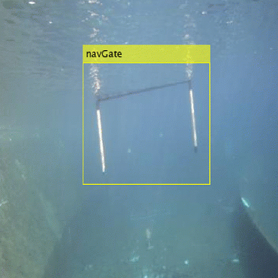
You need labelled images to perform a supervised learning approach. Hence the next step will be to label the objects of interest in the dataset.
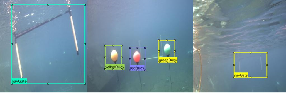
A. Create Ground Truth
With Ground Truth Labeler app or the Video Labeler app, you can label the objects, by using the in-built algorithms of the app or by integrating your own custom algorithms within the app. To create the ground truth in this example, we used the Ground Truth Labeler app, but you can achieve the same results and workflow with the Video Labeler app as well.
Once you have labelled images, you export the ground truth as a ground truth data object for each train, test, and validation dataset. Next you create the training data from the ground truth object by using the function objectDetectorTrainingData. You feed this training data in your network.
trainingData = objectDetectorTrainingData(gTruthResizedTrain,'SamplingFactor',1,...
    'WriteLocation','TrainingData');
To learn how you can implement the above steps, check out the video linked below.
III. Design & Train YOLOv2 Network
Now your data is ready. Let’s talk about the neural network.
So, what is a YOLOv2 Network? – You only look once (YOLO) is an object detection system targeted for real-time processing. It uses a single stage object detection network which is faster than other two-stage deep learning object detectors, such as regions with convolutional neural networks (Faster R-CNNs).
The YOLOv2 model runs a deep learning CNN on an input image to produce network predictions. The object detector decodes the predictions and generates bounding boxes.
A. Design YOLOv2 network layers
You can design a custom YOLOv2 model layer by layer from scratch. The model should always start with an input layer, followed by the detection subnetwork containing a series of Convolutional, Batch normalization, and ReLu (Rectified Linear Unit) layers. These layers are then connected the MATLAB’s inbuilt yolov2TransformLayer and yolov2OutputLayer.
yolov2TransformLayer transforms the raw CNN output into a form required to produce object detections. yolov2OutputLayer defines the anchor box parameters and implements the loss function used to train the detector.

Following the above approach, you use the imageInputLayer function to define the image input layer with minimum image size (128x128x3 used here). Use your best judgement based on the dataset and objects that need to be detected.
inputLayer = imageInputLayer([128 128 3],'Name','input','Normalization','none');
filterSize = [3 3];
Next is the middle layers. Following the basic approach of YOLO9000 paper, use a repeated batch of Convolution2dLayer, Batch Normalization Layer, RelU Layer, and Max Pooling Layer.
middleLayers = [
    convolution2dLayer(filterSize, 16, 'Padding', 1,'Name','conv_1',...
    'WeightsInitializer','narrow-normal')
    batchNormalizationLayer('Name','BN1')
    reluLayer('Name','relu_1')
    maxPooling2dLayer(2, 'Stride',2,'Name','maxpool1')
    convolution2dLayer(filterSize, 32, 'Padding', 1,'Name', 'conv_2',...
    'WeightsInitializer','narrow-normal')
    batchNormalizationLayer('Name','BN2')
    reluLayer('Name','relu_2')
    maxPooling2dLayer(2, 'Stride',2,'Name','maxpool2')
    convolution2dLayer(filterSize, 64, 'Padding', 1,'Name','conv_3',...
    'WeightsInitializer','narrow-normal')
    batchNormalizationLayer('Name','BN3')
    reluLayer('Name','relu_3')
    maxPooling2dLayer(2, 'Stride',2,'Name','maxpool3')
    convolution2dLayer(filterSize, 128, 'Padding', 1,'Name','conv_4',...
    'WeightsInitializer','narrow-normal')
    batchNormalizationLayer('Name','BN4')
    reluLayer('Name','relu_4')
    ];
At the end combine the initial & middle layers and convert into a layer graph object in order to manipulate the layers. You will use this layer graph for assembling the final network in step c below.
lgraph = layerGraph([inputLayer; middleLayers]);
Another parameter you require is the number of Classes. You should calculate it based on your Input data.
numClasses = size(trainingData,2)-1;
B. Define Anchor boxes
Before assembling the final network, you have the concept of anchor boxes in YOLO architecture. Anchor boxes are a set of predefined bounding boxes of a certain height and width. They are defined to capture the scale and aspect ratio of specific object classes you want to detect and are typically chosen based on object sizes in your training datasets. You can define several anchor boxes, each for a different object size. The use of anchor boxes enables a network to detect multiple objects, objects of different scales, and overlapping objects. You can study details about the Basics of anchor boxes here.
The anchor boxes are selected based on the scale and size of objects in the training data. You can Estimate Anchor Boxes Using Clustering to determine a good set of anchor boxes based on the training data. Using this procedure, the anchor boxes for the dataset used in this example are:
Anchors = [43 59
    18 22
    23 29
    84 109];
C. Assemble YOLOv2 network
The final step is to assemble all our above pieces of the network in a YOLOv2 architecture, using the function yolov2Layers. This function adds an inbuilt subnetwork of YOLO layers along with yolov2Transform and yolov2OutputLayer.
lgraph = yolov2Layers ([128 128 3],numClasses,Anchors,lgraph,'relu_4');
‘relu_4’ is the feature extraction layer. The features extracted from this layer are given as input to the YOLO v2 object detection subnetwork. You can specify any network layer except the fully connected layer as the feature layer.
You can visualize the lgraph using the network analyzer app.
analyzeNetwork(lgraph);

D. Train the Network
You can train the network once you have your layers ready. You now want to work on your model’s training options.
For training a network you always provide the algorithm with some training options. These options guide the network about how the network should learn. Changing with these options can help you to modify the network’s performance.
Learning Rate, mini batch size, and no of epochs are some of the important training options to consider. These help you decide what should be the learning speed of your network and how much data sample your network should train on, in each round of training.
For this example, based on the size of the data set I trained the network with the solver – stochastic gradient descent for 80 epochs with initial learning rate of 0.001 and mini-batch size of 16. Here I performed lower learning rate to give more time for training considering the size of data and adjusting the epoch and mini-batch size. You should modify the options based on your dataset.
options = trainingOptions('sgdm', ...
        'InitialLearnRate',0.001, ...
        'Verbose',true,'MiniBatchSize',16,'MaxEpochs',80,...
        'Shuffle','every-epoch','VerboseFrequency',50, ...
        'DispatchInBackground',true,...
        'ExecutionEnvironment','auto');
Once you have your training data, network, and training options, train the detector using the YOLOv2 training function – trainYOLOv2ObjectDetector
[detectorYolo2, info] = trainYOLOv2ObjectDetector(trainingData,lgraph,options);
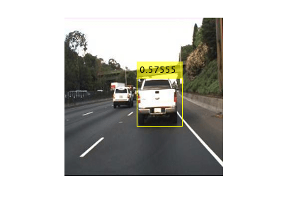
E. Detect output with the detector
Once you have the detector you can check the results visually, by running the detector through the images in the validation dataset.
You can do so by first creating a table to hold the results.
results = table('Size',[height(TestData) 3],...
    'VariableTypes',{'cell','cell','cell'},...
    'VariableNames',{'Boxes','Scores', 'Labels'});
Then Initialize a Deployable Video Player to view the image stream.
depVideoPlayer = vision.DeployableVideoPlayer;
And then loop through all the images in the Validation set.
for i = 1:height(ValidationData)

    % Read the image
    I = imread(ValidationData.imageFilename{i});

    % Run the detector.
    [bboxes,scores,labels] = detect(detectorYolo2,I);

    %
    if ~isempty(bboxes)
        I = insertObjectAnnotation(I,'Rectangle',bboxes,cellstr(labels));
        depVideoPlayer(I);
        pause(0.1);

    end

    % Collect the results in the results table
    results.Boxes{i} = floor(bboxes);
    results.Scores{i} = scores;
    results.Labels{i} = labels;

end
F. Evaluate
Once you have a trained detector and have visually confirmed the detection on Validation data, you can compute numerical evaluation metrics and plot the results on the test data.
MATLAB offers built-in functions evaluateDetectionPrecision and evaluateDetectionMissRate to evaluate precision metrics and miss rate metrics respectively.
[ap, recall, precision] = evaluateDetectionPrecision(results, TestData(:,2:end),threshold);

[am,fppi,missRate] = evaluateDetectionMissRate(results, TestData(:,2:end),threshold);
When it comes to the miss rate and precision, an important parameter used is threshold. The threshold parameter determines the extent of overlap of the bounding box around an object of interest given by the detector over the bounding box of the same object in the ground truth. It is calculated as the Intersection over Union (IoU) or Jaccard index. As shown in the plots below for the same detection and ground truth data, changing the value of the threshold parameter drastically changes the value of the evaluation metric. Pick an overlap threshold value that best suits your application and keep in mind a higher threshold means you are expecting your detection results to overlap a larger area of the ground truth.
Threshold value 0.7

Threshold value 0.3

Check out the video below to learn how you can work through above described steps of Designing and Training YOLOv2 network.
IV. Import Python based model
Another approach for training the network is importing the Python or other 3rd party developed models in MATLAB. One way is to follow the below workflow:
Convert your Python into ONNX model –> import the ONNX model into MATLAB
To learn more how you can import the pre-trained YOLOv2 ONNX model into MATLAB and train it on your custom dataset check out the below blog & video.
Blog: YOLOv2 Object Detection from ONNX Model in MATLAB
Video: Import Pretrained Deep Learning Networks into MATLAB
Summary
Some key takeaways:
- You can use Ground Truth Labeler app or Video Labeler app to label your images either using app’s inbuilt algorithms or importing your own custom algorithms. Check out this doc page to choose the appropriate labeling tool for your application
- You can design a neural network using MATLAB’s inbuilt layers functions
- The yolov2Layers functions adds subnetwork of yolo layers at the end of your own network or pretrained network
- You can import the Python based ONNX models in MATLAB and retrain them on your own dataset
Hence, we learned here that you can simplify the difficulty of working with different platforms by developing a complete Object Detection model in a single environment of MATLAB. Check out the next post to learn how you can deploy this model on your NVIDIA Jetson.
- Category:
- Data Science,
- Robotics,
- Video,
- Workflow


Comments
To leave a comment, please click here to sign in to your MathWorks Account or create a new one.