
Apply AI with New R2023a Examples
There are many new examples in the documentation of the latest MATLAB release (R2023a) that show how to use and apply the newest machine learning and deep learning features. Feel free to take a deep dive into the machine learning release notes and deep learning release notes to explore all new features and examples.
In this blog post, I will show highlights from three new examples that apply deep learning:
Note: This section of the blog post describes an example that was updated in R2023b. Check out the updated example Detect Defects on Printed Circuit Boards Using YOLOX Network, which uses a YOLOX instead of a YOLO v4 object detector.
Visual inspection is the image-based inspection of parts where a camera scans the part under test for both failures and quality defects. Visual inspection systems with high-resolution cameras efficiently detect microscale or even nanoscale defects that are difficult for human eyes to pick up.
Here, I will show you highlights from the documentation example Detect Defects on Printed Circuit Boards (PCBs) Using YOLO v4 Network. PCBs contain individual electronic devices and their connections. Defects in PCBs can result in poor performance or product failures. By detecting these defects, production lines can remove faulty PCBs and ensure that electronic devices are of high quality.
This example shows how to detect, localize, and classify defects on PCBs using a YOLOv4 deep neural network. I will mainly highlight the MATLAB tools that allow you to streamline the visual inspection of PCBs and focus on the application, rather than spending too much time on data management and creating a deep learning network.
Figure: Image of visually inspected PCB that shows missing holes
Figure: Scalogram of EEG time series
Define a network that uses a time-frequency transformation of the input signal for classification.
Figure: Confusion matrix chart for EEG classification
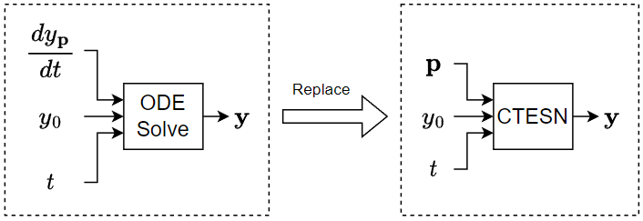 Figure: Replace ODE solver with a continuous-time echo state network.
You can apply the methods shown in the example if you need to solve an ODE in a model multiple times with different parameters. To save computational resources, instead of approximating the solution using an ODE solver within the system, you can train a neural network using a collection of automatically-derived solutions and then, incorporate the neural network in your model. A CTESN model typically evaluates faster than an ODE solver.
Figure: Replace ODE solver with a continuous-time echo state network.
You can apply the methods shown in the example if you need to solve an ODE in a model multiple times with different parameters. To save computational resources, instead of approximating the solution using an ODE solver within the system, you can train a neural network using a collection of automatically-derived solutions and then, incorporate the neural network in your model. A CTESN model typically evaluates faster than an ODE solver.
Prepare Training Data
MATLAB provides functions for preparing data for object detection, some of which are presented in this table:| Functionality | MATLAB Function | More Details |
| Data management | imageDatastore | Read and manage training images. |
| fileDatastore | Read and manage annotation data. | |
| combine | Combine multiple datastores. | |
| Transform data | transform | Transform data in datastores to (1) resize images and bounding boxes to the size of the input network and (2) augment (e.g., horizontal flip and scale) input data. |
| Estimate anchor boxes | estimateAnchorBoxes | Estimate a specified number of anchor boxes based on the size of objects in the preprocessed training data. |
Create Detector
Instead of creating a deep learning model from scratch, you can get a pretrained model, which you can modify and retrain to adapt to your task. You can get the YOLOv4 object detector in just one line of code by using the yolov4ObjectDetector function.detectorToTrain = yolov4ObjectDetector("tiny-yolov4-coco",classNames, ...
anchorBoxes, InputSize=inputSize);
After you get the object detector, use the trainYOLOv4ObjectDetector function to train it.
Inspect Single Image
The detect function can predict bounding boxes, labels, and class-specific confidence scores for each bounding box. Use detect to inspect a single image and display the results.[bboxes,scores,labels] = detect(detector,sampleImage);
imshow(sampleImage)
showShape("rectangle",bboxes,Label=labels);
title("Predicted Defects")
For this specific image three missing holes are detected on the PCB, as shown in the figure below. Imagine the implications in the mass production of PCBs…

Inspect Multiple Images
As easily as detecting defects on a single PCB, the detect function can find defects on all the PCB images in the data store. Then, you can evaluate the trained object detector. Detect the bounding boxes for all test images.detectionResults = detect(detector,dsTest);Calculate the average precision score for each class by using the evaluateDetectionPrecision function. Precision quantifies the ability of the detector to correctly classify objects. Also calculate the recall and precision values from each detected defect. Recall quantifies the ability of the detector to detect all relevant objects for a class.
[averagePrecision,recall,precision] = evaluateDetectionPrecision(detectionResults,dsTest);
More resources
- Check out more visual inspection examples.
- Check out how C-CORE and Equinor developed automated software with MATLAB to analyze satellite radar imagery with deep learning.
- Check out the Computer Vision Toolbox Automated Visual Inspection Library, which enables you to train, calibrate, and evaluate stat-of-the-art anomaly detectors.
Training Data Preparation
In addition to the MATLAB tools for data management shown in the visual inspection example (and others), MATLAB also provides a datastore for tabular text files, which helps manage the EEG time series in this example.Deep Learning Network
The convolutional network predicts the class of the EEG data based on the squared magnitude of the continuous wavelet transform (CWT), which you can easily compute by using the cwt function. This squared magnitude is also known as a scalogram. The scalogram is an ideal time-frequency transformation for time series data like EEG waveforms, which feature both slowly-oscillating and transient phenomena.
netSPN =
    [sequenceInputLayer(1,"MinLength",4097,"Name","input","Normalization","zscore")
    convolution1dLayer(5,1,"stride",2)
    cwtLayer("SignalLength",2047,"IncludeLowpass",true,"Wavelet","amor")
    maxPooling2dLayer([5,10])
    convolution2dLayer([5,10],5,"Padding","same")
    maxPooling2dLayer([5,10])
    batchNormalizationLayer
    reluLayer
    convolution2dLayer([5,10],10,"Padding","same")
    maxPooling2dLayer([2,4])
    batchNormalizationLayer
    reluLayer
    flattenLayer
    globalAveragePooling1dLayer
    dropoutLayer(0.4)
    fullyConnectedLayer(3)
    softmaxLayer
  classificationLayer("Classes",unique(trainLabelsSPN),"ClassWeights",classwghts)
    ];
Unlike deep learning networks that use the magnitude or squared magnitude of the CWT (scalogram) as a preprocessing step, this example uses a differentiable scalogram layer (cwtLayer) . With a differentiable scalogram layer inside the network, you can put learnable operations before and after the scalogram. Layers of this type significantly expand the architectural variations that are possible with time-frequency transforms.
Classification Results
Visualize the classification results with a confusion matrix chart. The confusion chart shows good performance on the test set. The row summaries in the confusion chart show the model's recall, while the column summaries show the precision. Both recall and precision generally fall between 95 and 100 percent.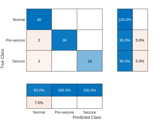
More Resources
Check out the following links, to see how MATLAB users have applied machine learning and deep learning to EEG-based BMIs and epileptic seizure detection:- Using Machine Learning to Predict Epileptic Seizures from EEG Data
- Dutch Epilepsy Clinics Foundation Automates the Detection and Diagnosis of Epileptic Seizures
- UT Austin Researchers Convert Brain Signals to Words and Phrases Using Wavelets and Deep Learning
Reduced Order Modeling with AI
Reduced Order Modeling (ROM) is a technique for reducing the computational complexity or storage requirement of a computer model, while preserving the expected fidelity within a controlled error. High-fidelity non-linear models can take hours or even days to simulate. This causes a significant computational challenge for many engineering teams. AI-based reduced-order models can significantly speed up simulations and analysis of higher-order large-scale systems. AI enables to create a model from measured data of your component, so you get the right answer in an accurate, dynamic, and low-cost way. Even if you already have a high-fidelity first-principles model, you can use data-driven models to create a surrogate model that is potentially simpler and simulates faster. A faster but equally accurate model can help you progress as you design, test, and deploy your system. To learn more about ROM using AI, check out our previous blog post and this video.Example Overview
You can train AI models using various techniques, such as LSTMs and Neural ODEs. This new example shows how to perform reduced order modeling using a continuous-time echo state network (CTESN). This neural network is a type of recurrent neural network (RNN), as is an LSTM, which uses a reservoir computing framework to project signals from higher dimensional spaces.
Figure: Replace ODE solver with a continuous-time echo state network.
You can apply the methods shown in the example if you need to solve an ODE in a model multiple times with different parameters. To save computational resources, instead of approximating the solution using an ODE solver within the system, you can train a neural network using a collection of automatically-derived solutions and then, incorporate the neural network in your model. A CTESN model typically evaluates faster than an ODE solver.
Conclusion
I hope that the above brief description of the three new examples sparked your curiosity to try them out and explore other new AI features and examples in MATLAB R2023. Comment here to talk about your exciting AI applications and how you are going to take advantage of the latest MATLAB AI features.- Category:
- AI Application,
- Deep Learning,
- New features


Comments
To leave a comment, please click here to sign in to your MathWorks Account or create a new one.