
Using MATLAB Graphics from Simulink
Today we're going to take a break from the math behind parametric curves and take a look at using MATLAB Graphics from Simulink.
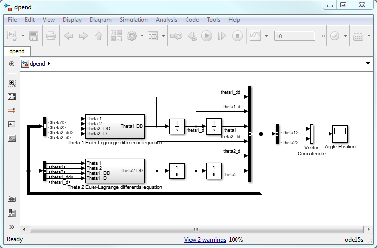
Combining MATLAB Graphics with Simulink is a very powerful technique for visualizing simulations, but it can be hard to figure out how to get started. Today we’re going to work through a simple example. We’ll start with double pendulum example that Guy Rouleau built as a benchmark for his blog post about SimMechanics. You can get it from the File Exchange.
We're going to modify it so that it creates a figure window which shows the pendulum animating while the simulation runs.
We'll do this in two steps. First we'll create a MATLAB class which implements all of the graphics. Next we'll use that class from Simulink. The reason for doing it in two steps is that it makes it easier to debug the graphics before we start integrating it with Simulink.
Contents
Creating the parts of the visualization
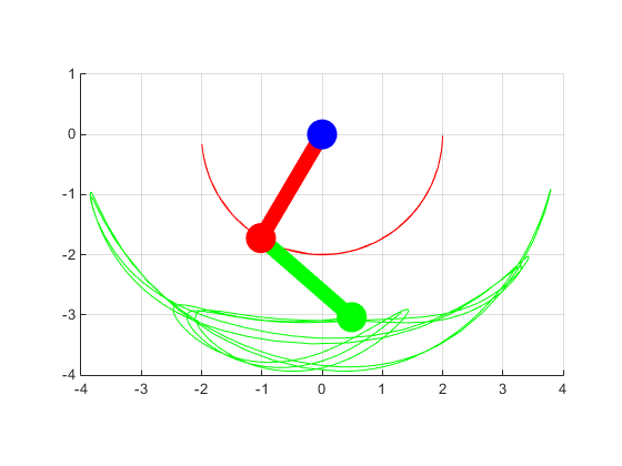
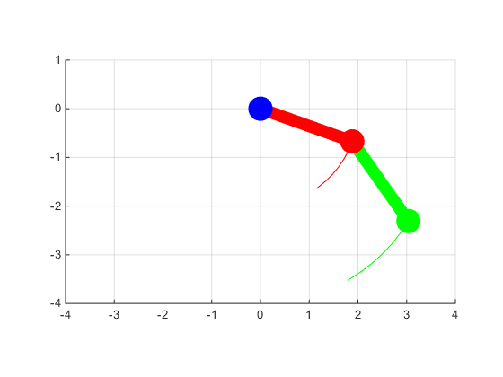
If you look at the picture above, you can see that we need three parts to represent the pendulum, and two objects to represent the traces.
The traces are easy. That’s exactly what the new animatedline object is for.
trace1 = animatedline('Color', 'red');
trace2 = animatedline('Color', 'green');
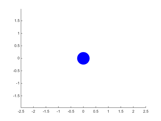
The blue anchor point is also pretty easy. It’s just the punchline of a very old MATLAB graphics joke:
How do you draw a circle in MATLAB?
The answer is the rectangle command, of course! If we call the rectangle function with a Curvature property, it will round the corners off. If the value of the Curvature is [1 1], then the corners will be completely rounded off, and we'll get a circle!
circle = rectangle('Curvature',[1 1]);
r = .5;
circle.Position = [-r/2, -r/2, r, r];
circle.EdgeColor = 'none';
circle.FaceColor = 'blue';
axis equal
xlim([-2.5 2.5])
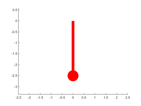
The arms are a little trickier. When they’re hanging down, we can draw them using two rectangles (one of which is really a circle), but we're going to want them to swing. The hgtransform object is the solution to that. The hgtransform object has a Matrix property which we can use to move its children around.
Here's a simple function which shows how to create an arm from an hgtransform and two rectangles.
%
% File: createArm.m
%
function p = createArm(w, r, len, col)
% Creates the geometry for one pendulum.
  p = hgtransform;
  l = rectangle('Parent',p);
  l.Position = [-w/2, -len, w, len];
  l.FaceColor = col;
  l.EdgeColor = 'none';
  c = rectangle('Parent',p,'Curvature',[1 1]);
  c.Position = [-r/2, -(len+r/2), r, r];
  c.EdgeColor = 'none';
  c.FaceColor = col;
end
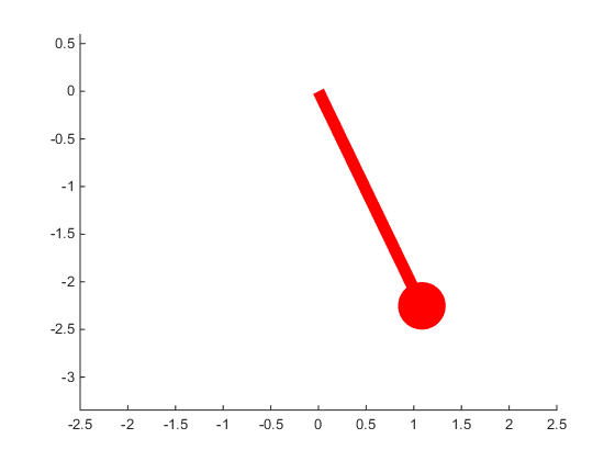
cla
arm = createArm(.125,r,2.5,'red');
axis equal
axis manual
Now we can change the hgtransform object's Matrix property to make the arm rotate. That's easy to do by using the makehgtform function.
arm.Matrix = makehgtform('zrotate',pi/7);
Creating a DoublePendulum class
If we put these parts together, we get a class which looks something like the following:
%
% File: DoublePendulum.m
%
classdef DoublePendulum < handle
  % A class for implementing a MATLAB Graphics visualization of the
  % Simulink model of the double pendulum which Guy Rouleau shared in
  % File Exchange posting 23126.
  %
  properties (SetAccess=private)
    Arms    = gobjects(1,2);
    Traces  = gobjects(1,2);
    Lengths = [2 2];
    Angles  = [0 0];
    BallWidth = .5;
    ArmWidth = .25;
  end
  %
  % Public methods
  methods
    function obj = DoublePendulum()
      obj.createGeometry();
      obj.updateTransforms();
    end
    function setAngles(obj, a1, a2)
    % Call this to change the angles.
      obj.Angles(1) = a1;
      obj.Angles(2) = a2;
      obj.addTracePoints();
      obj.updateTransforms();
    end
    function clearPoints(obj)
    % Call this to reset the traces.
      obj.Traces(1).clearpoints();
      obj.Traces(2).clearpoints();
    end
    function r = isAlive(obj)
    % Call this to check whether the figure window is still alive.
      r = isvalid(obj) && ...
          isvalid(obj.Arms(1)) && isvalid(obj.Arms(2)) && ...
          isvalid(obj.Traces(1)) && isvalid(obj.Traces(2));
    end
  end
  %
  % Private methods
  methods (Access=private)
    function createArm(obj, p, len, col)
    % Creates the geometry for one pendulum. This is basically a copy
    % of the function we created earlier.
      w = obj.ArmWidth;
      l = rectangle('Parent',p);
      l.Position = [-w/2, -len, w, len];
      l.FaceColor = col;
      l.EdgeColor = 'none';
      c = rectangle('Parent',p);
      r = obj.BallWidth;
      c.Position = [-r/2, -(len+r/2), r, r];
      c.Curvature = [1 1];
      c.EdgeColor = 'none';
      c.FaceColor = col;
    end
    function addTracePoints(obj)
    % Adds the current end points of the two pendulums to the traces.
      a1 = obj.Angles(1);
      a2 = obj.Angles(2);
      l1 = obj.Lengths(1);
      l2 = obj.Lengths(2);
      x1 =  l1*sin(a1);
      y1 = -l1*cos(a1);
      x2 = x1 + l2*sin(a1+a2);
      y2 = y1 - l2*cos(a1+a2);
      obj.Traces(1).addpoints(x1,y1);
      obj.Traces(2).addpoints(x2,y2);
    end
    function createGeometry(obj)
    % Creates all of the graphics objects for the visualization.
      col1 = 'red';
      col2 = 'green';
      col3 = 'blue';
      fig = figure;
      ax = axes('Parent',fig);
      % Create the traces
      obj.Traces(1) = animatedline('Parent', ax, 'Color', col1);
      obj.Traces(2) = animatedline('Parent', ax, 'Color', col2);
      % Create the transforms
      obj.Arms(1) = hgtransform('Parent', ax);
      obj.Arms(2) = hgtransform('Parent', obj.Arms(1));
      % Create the arms
      createArm(obj, obj.Arms(1), obj.Lengths(1), col1);
      createArm(obj, obj.Arms(2), obj.Lengths(2), col2);
      % Create a blue circle at the origin.
      c = rectangle('Parent',ax);
      r = obj.BallWidth;
      c.Position = [-r/2, -r/2, r, r];
      c.Curvature = [1 1];
      c.EdgeColor = 'none';
      c.FaceColor = col3;
      % Initialize the axes.
      maxr = sum(obj.Lengths);
      ax.DataAspectRatio = [1 1 1];
      ax.XLim = [-maxr maxr];
      ax.YLim = [-maxr 1];
      grid(ax,'on');
      ax.SortMethod = 'childorder';
    end
    function updateTransforms(obj)
    % Updates the transform matrices.
      a1 = obj.Angles(1);
      a2 = obj.Angles(2);
      offset = [0 -obj.Lengths(1) 0];
      obj.Arms(1).Matrix = makehgtform('zrotate', a1);
      obj.Arms(2).Matrix = makehgtform('translate', offset, ...
                                       'zrotate', a2);
    end
  end
end
Notice the createGeometry method which creates each of the parts we talked about earlier. It creates two traces (one red and one green), followed by two arms (again, one red and one green), and then adds a blue circle at the origin.
Also notice the setAngles method. That adds a new angle to each of the traces, and calls makehgtform to rotate each of the two arms.
Now we can create an instance of this class at the MATLAB command line, and use the setAngles method to make it move.
cla
h = DoublePendulum();
for a=pi/5:.1:2*pi/5
  h.setAngles(a,-a/2);
end
Once we have it working, we're ready to move on to the next step.
Connecting to Simulink
The final step is to connect it to Simulink. There are a couple of different ways to do this. We’re going to do it with an S-function. We drag a Level-2 MATLAB S-Function block out of the library, connect it to the same signal as the scope labeled "Angle Position", and set its S-function to the following:
%
% File: doublePendulumSFunction.m
%
function doublePendulumSFunction(block)
% Level-2 MATLAB file S-function for visualizing a double pendulum.
  setup(block)
end
%
% Called when the block is added to a model.
function setup(block)
  %
  % 1 input port, no output ports
  block.NumInputPorts  = 1;
  block.NumOutputPorts = 0;
  %
  % Setup functional port properties
  block.SetPreCompInpPortInfoToDynamic;
  %
  % The input is a vector of 2 angles
  block.InputPort(1).Dimensions = 2;
  %
  % Register block methods
  block.RegBlockMethod('Start',   @Start);
  block.RegBlockMethod('Outputs', @Output);
  %
  % To work in external mode
  block.SetSimViewingDevice(true);
end
%
% Called when the simulation starts.
function Start(block)
  %
  % Check to see if we already have an instance of DoublePendulum
  ud = get_param(block.BlockHandle,'UserData');
  if isempty(ud)
    vis = [];
  else
    vis = ud.vis;
  end
  %
  % If not, create one
  if isempty(vis) || ~isa(vis,'DoublePendulum') || ~vis.isAlive
    vis = DoublePendulum();
  else
    vis.clearPoints();
  end
  ud.vis = vis;
  %
  % Save it in UserData
  set_param(block.BlockHandle,'UserData',ud);
end
%
% Called when the simulation time changes.
function Output(block)
  if block.IsMajorTimeStep
    % Every time step, call setAngles
    ud = get_param(block.BlockHandle,'UserData');
    vis = ud.vis;
    if isempty(vis) || ~isa(vis,'DoublePendulum') || ~vis.isAlive
      return;
    end
    vis.setAngles(block.InputPort(1).Data(1), ...
                  block.InputPort(1).Data(2));
  end
end
There are three pieces to this S-Function.
- The setup function gets called when the block gets loaded. This tells Simulink how to connect the block up to the rest of the model, and it registers the two functions which do the real work.
- The function Start gets called when the simulation starts. All it does is create an instance of the DoublePendulum class we defined above, and saves it away in the block's UserData.
- The function Output gets called whenever the simulation updates the block's inputs. All we need to do here is call the setAngles method on our DoublePendulum class. It will do all the work of updating our visualization.
Results
And that's it! Just press the Run button, and away we go with our pendulum swinging around wildly.
Have you got Simulink models which could benefit from custom MATLAB graphics like this?
- Category:
- Animation

