Rooting Around in MATLAB – Part 3

I recently wrote a pair of posts (1 and 2) about finding roots of equations, and how you might use MATLAB to explore this topic with emphasis on the method of fixed point iteration.

Contents

Set Up

clear all
close all

Example Reminder

Let me restate the example function. Let's start with a simple cubic polynomial f(x)

which we define using an anonymous function.

f = @(x) x.^3 + x - 1;
fplot(f,[-2 2])
title f
grid on

First Fixed Point Iteration Attempt

Previously we rewrote f(x)=0 so that x was alone on one side of the equation.

g1 = @(x) 1 - x.^3;

This function, g1(x) did not help find the root between 0 and 1 - every step took us further away from the solutions we found with roots and fzero.

fzsolution = fzero(f,0.5)

fzsolution =
      0.68233

Second Way to Rewrite Equation

There's another way we can write the equation for the fixed point. Remember, we want to rearrange f(x)=0 into something like g2(x)=x. We have already tried g1 = 1 - x^3. We can also rewrite the equation as

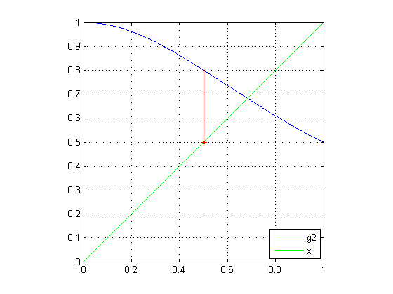
g2 = @(x) 1./(x.^2+1);
fplot(g2,[0 1]);
hold on
straightLine = @(x) x;
fplot(straightLine, [0 1], 'g')
legend('g2','x','Location','SouthEast')
grid on
axis equal, axis([0 1 0 1])

Let's Iterate

Following the same idea from the last post, we now iterate, finding successive guesses of x, computing the value of g2(x), setting this value to be the next estimate of x, etc.

Let's Try to "Zero" in on the Solution

First, we'll select a starting value x = 0.5, and y, from the straight line also at 0.5.

x(1) = 0.5;
y(1) = x(1);
x(2) = x(1);
y(2) = g2(x(2));

And let's plot the trajectory of the solutions, starting with the first point.

plot(x,y,'r',x(1),y(1),'r*')

First Iteration

As described in the previous post, I now set the current value of g2 to the new x value, sliding onto the straight line, and then calculate the next value of g2 from this new value for x. And plot it.

x(3) = y(2);
y(3) = y(2);
x(4) = x(3);
y(4) = g2(x(4));
plot(x,y,'r')

Second Iteration

Here's the second iteration.

n = 5;
x(n) = y(n-1);
y(n) = y(n-1);
x(n+1) = x(n);
y(n+1) = g2(x(n+1));
plot(x,y,'r')

Third Iteration

And the third.

n = 7;
x(n) = y(n-1);
y(n) = y(n-1);
x(n+1) = x(n);
y(n+1) = g2(x(n+1));
plot(x,y,'r')

A Few More Rounds

Let's do a few more iterations and preallocate the arrays instead of growing them. And yes, I know in this post I kept overplotting lines successively. I didn't want us to get distracted by managing the plots.

x(9:22) = NaN;
y(9:22) = NaN;
for n = 9:2:21
    x(n) = y(n-1);
    y(n) = y(n-1);
    x(n+1) = x(n);
    y(n+1) = g2(x(n+1));
end
plot(x,y,'r')
hold off

Fixed Point Found!

We appear to be converging on a fixed point, since after iterating, the final values for x and g2(x) (which is y) are getting quite close to each other.

final = [ x(end) y(end) fzsolution]

final =
      0.68039      0.68356      0.68233

Wrapping Up the Series of Posts

This post completes this series of posts on fixed point iteration. There is, of course, more that you could do in a class. For example, you might explore what characteristics of the functions g1 and g2 made the fixed point iteration strategy behave differently. Perhaps look at first derivatives?

Here's the recap of the series

Is this sort of tutorial relevant to your work, especially if you are teaching? How about the incorporation of the visualization during the exploration? Let me know your thoughts here.

Get the MATLAB code

Published with MATLAB® 7.8