 Cleve’s Corner: Cleve Moler on Mathematics and Computing
 The MATLAB Blog
 Guy on Simulink
 MATLAB Community
 Artificial Intelligence
 Developer Zone
 Stuart’s MATLAB Videos
 Behind the Headlines
 File Exchange Pick of the Week
 Hans on IoT
 Student Lounge
 MATLAB ユーザーコミュニティー
 Startups, Accelerators, & Entrepreneurs
 Autonomous Systems
 Quantitative Finance
 MATLAB Graphics and App Building
Process “Big Data” in MATLAB with mapreduce
Today I’d like to introduce guest blogger Ken Atwell who works for the MATLAB Development team here at MathWorks. Today, Ken will be discussing with you the MapReduce programming technique now available in the R2014b release of MATLAB. MapReduce provides a way to process large amounts of file-based data on a single computer in MATLAB. For very large data sets, the same MATLAB code written using MapReduce can also be run on the "big data" platform, Hadoop®.
Contents
About the data
The data set we will be using consists of records containing flight performance metrics for USA domestic airlines for the years 1987 through 2008. Each year consists of a separate file. If you have experimented with "big data" before, you may already be familiar with this data set. The full data set can be downloaded from here. A small subset of the data set, airlinesmall.csv, is also included with MATLAB® to allow you to run this and other examples without downloading the entire data set.
Introduction to mapreduce
MapReduce is a programming technique that is used to "divide and conquer" big data problems. In MATLAB, the mapreduce function requires three input arguments:
- A datastore for reading data into the "map" function in a chunk-wise fashion.
- A "map" function that operates on the individual chunks of data. The output of the map function is a partial calculation. mapreduce calls the map function one time for each chunk of data in the datastore, with each call operating independently from other map calls.
- A "reduce" function that is given the aggregate outputs from the map function. The reduce function finishes the computation begun by the map function, and outputs the final answer.
This is an over-simplification to some extent, since the output of a call to the map function can be shuffled and combined in interesting ways before being passed to the reduce function. This will be examined later.
Use mapreduce to perform a computation
Let's look at a straightforward example to illustrate how mapreduce is used. In this example we want to find the longest flight time out of all the flights recorded in the entire airline data set. To do this we will:
- Create a datastore object to reference our airline data set
- Create a "map" function that computes the maximum flight time in each chunk of data in the datastore.
- Create a "reduce" function that computes the maximum value among all of the maxima computed by the calls to the map function.
Create a datastore
datastore is used to access collections of tabular text files stored on a local disk, or the Hadoop® Distributed File System (HDFS™). It is also the mechanism for providing data in a chunk-wise manner to the map calls when using mapreduce. A previous blog post explained how datastore works and how it is used for reading collections of data that are too large to fit in memory.
Let's create our datastore and first preview the data set. This allows us to peek into the data set, and identify the format of the data and the columns that contain the data we are interested in. The preview will normally provide a small chunk of data that contains all the columns present in the data set, although I will only show a handful of columns to make our article more readable.
ds = datastore('airlinesmall.csv', 'DatastoreType', 'tabulartext', ...
    'TreatAsMissing', 'NA');
data = preview(ds);
data(:,[1,2,3,9,12])
ans =
    Year    Month    DayofMonth    UniqueCarrier    ActualElapsedTime
    ____    _____    __________    _____________    _________________
    1987    10       21            'PS'              53
    1987    10       26            'PS'              63
    1987    10       23            'PS'              83
    1987    10       23            'PS'              59
    1987    10       22            'PS'              77
    1987    10       28            'PS'              61
    1987    10        8            'PS'              84
    1987    10       10            'PS'             155
For the computation we are looking to perform, we only need to look at the "ActualElapsedTime" column: it contains the actual flight time. Let's configure our datastore to only provide this one column to our map function.
ds.SelectedVariableNames = {'ActualElapsedTime'};
Create a map function
Now we will write our map function (MaxTimeMapper.m). Three input arguments will be provided to our map function by mapreduce:
- The input data, "ActualElapsedTime", which is provided as a MATLAB table by datastore.
- A collection of configuration and contextual information, info. This can be ignored in most cases, as it is here.
- An intermediate data storage object, where the results of the calculations from the map function are stored. Use the add function to add key/value pairs to this intermediate output. In this example, we have arbitrarily chosen the name of the key ('MaxElapsedTime').
Our map function finds the maximum value in the table 'data', and saves a single key ('MaxElapsedTime') and corresponding value to the intermediate data storage object. We will now go ahead and save the following map function (MaxTimeMapper.m) to our current folder.
function MaxTimeMapper(data, ~, intermediateValuesOut)
maxTime = max(data{:,:});
add(intermediateValuesOut, 'MaxElapsedTime', maxTime);
end
Create a reduce function
Next, we create the reduce function (MaxTimeReducer.m). Three input arguments will also be provided to our reduce function by mapreduce:
- A set of input "keys". Keys will be discussed further below, but they can be ignored in some simple problems, as they are here.
- An intermediate data input object that mapreduce passes to the reduce function. This data is the output of the map function and is in the form of key/value pairs. We will use the hasnext and getnext functions to iterate through the values.
- A final output data storage object where the results of the reduce calculations are stored. Use the add and addmulti functions to add key/value pairs to the output.
Our reduce function will receive a list of values associated with the 'MaxElapsedTime' key which were generated by the calls to our map function. The reduce function will iterate through these values to find the maximum. We create the following reduce function (MaxTimeReducer.m) and save it to our current folder.
function MaxTimeReducer(~, intermediateValuesIn, finalValuesOut)
maxElapsedTime = -inf;
while hasnext(intermediateValuesIn)
   maxElapsedTime = max(maxElapsedTime, getnext(intermediateValuesIn));
end
add(finalValuesOut, 'MaxElapsedTime', maxElapsedTime);
end
Run mapreduce
Once the map and reduce functions are written and saved in our current folder, we can call mapreduce and reference the datastore, map function, and reduce function to run our calculations on our data. The readall function is used here to display the results of the MapReduce algorithm.
result = mapreduce(ds, @MaxTimeMapper, @MaxTimeReducer);
readall(result)
Parallel mapreduce execution on the local cluster:
********************************
*      MAPREDUCE PROGRESS      *
********************************
Map   0% Reduce   0%
Map 100% Reduce 100%
ans =
          Key           Value
    ________________    ______
    'MaxElapsedTime'    [1650]
If Parallel Computing Toolbox is available, MATLAB will automatically start a pool and parallelize execution of the map functions. Since the number of calls to the map function by mapreduce corresponds to the number of chunks in the datastore, parallel execution of map calls may speed up overall execution.
Use of keys in mapreduce
The use of keys is an important feature of mapreduce. Each call to the map function can add intermediate results to one or more named "buckets", called keys.
If the map function adds values to multiple keys, this leads to multiple calls to the reduce function, with each reduce call working on only one key's intermediate values. The mapreduce function automatically manages this data movement between the map and reduce phases of the algorithm.
Calculating group-wise metrics with mapreduce
The behavior of the map function in this case is more complex and will illustrate the benefits to using multiple keys to store your intermediate data. For every airline found in the input data, use the add function to add a vector of values. This vector is a count of the number of flights for that carrier for each day in the 21+ years of data. The carrier code is the key for this vector of values. This ensures that all of the data for each carrier will be grouped together when mapreduce passes it to the reduce function.
Here's our new map function (CountFlightsMapper.m).
function CountFlightsMapper(data, ~, intermediateValuesOut)
dayNumber = days((datetime(data.Year, data.Month, data.DayofMonth) - datetime(1987,10,1)))+1;
daysSinceEpoch = days(datetime(2008,12,31) - datetime(19875,10,1))+1;
[airlineName, ~, airlineIndex] = unique(data.UniqueCarrier);
for i = 1:numel(airlineName)
   dayTotals = accumarray(dayNumber(airlineIndex==i), 1, [daysSinceEpoch, 1]);
   add(intermediateValuesOut, airlineName{i}, dayTotals);
end
end
The reduce function is less complex. It simply iterates over the intermediate values and adds the vectors together. At completion, it outputs the values in this accumulated vector. Note that the reduce function does not need to sort or examine the intemediateKeysIn values; each call to the reduce function by mapreduce only passes the values for one airline.
Here's our new reduce function (CountFlightsReducer.m).
function CountFlightsReducer(intermediateKeysIn, intermediateValuesIn, finalValuesOut)
daysSinceEpoch = days(datetime(2008,12,31) - datetime(1987,10,1))+1;
dayArray = zeros(daysSinceEpoch, 1);
while hasnext(intermediateValuesIn)
   dayArray = dayArray + getnext(intermediateValuesIn);
end
add(finalValuesOut, intermediateKeysIn, dayArray);
end
To run this new analysis, just reset the datastore and select the active variables of interest. In this case we want the date (year, month, day) and the airline carrier name. Once the map and reduce functions are written and saved in our current folder, mapreduce is called referencing the updated datastore, map function, and reduce function.
reset(ds);
ds.SelectedVariableNames = {'Year', 'Month', 'DayofMonth', 'UniqueCarrier'};

result = mapreduce(ds, @CountFlightsMapper, @CountFlightsReducer);
result = result.readall();
Parallel mapreduce execution on the local cluster:
********************************
*      MAPREDUCE PROGRESS      *
********************************
Map   0% Reduce   0%
Map 100% Reduce  50%
Map 100% Reduce 100%
Up until this point we have been only analyzing the sample data set (airlinesmall.csv). To look at the number of flights each day over the full dataset, let's load the results of running our new MapReduce algorithm on the entire data set.
load airlineResults
Visualizing the results
Before looking at the number of flights per day for the top 7 carriers, let us first apply a filter to the data to smooth out the effects of weekend travel. This would otherwise clutter the visualization.
lines = result.Value;
lines = horzcat(lines{:});
[~,sortOrder] = sort(sum(lines), 'descend');
lines = lines(:,sortOrder(1:7));
result = result(sortOrder(1:7),:);

lines(lines==0) = nan;
for carrier=1:size(lines,2)
    lines(:,carrier) = filter(repmat(1/7, [7 1]), 1, lines(:,carrier));
end
figure('Position',[1 1 800 800]);
plot(datetime(1987,10,1):caldays(1):datetime(2008,12,31),lines)
title ('Domestic airline flights per day per carrier')
xlabel('Date')
ylabel('Flights per day (7-day moving average)')

try
    carrierList = readtable('carriers.csv.txt', 'ReadRowNames', true);
    result.Key = cellfun(@(x) carrierList(x, :).Description, result.Key);
catch
end
legend(result.Key, 'Location', 'SouthOutside')
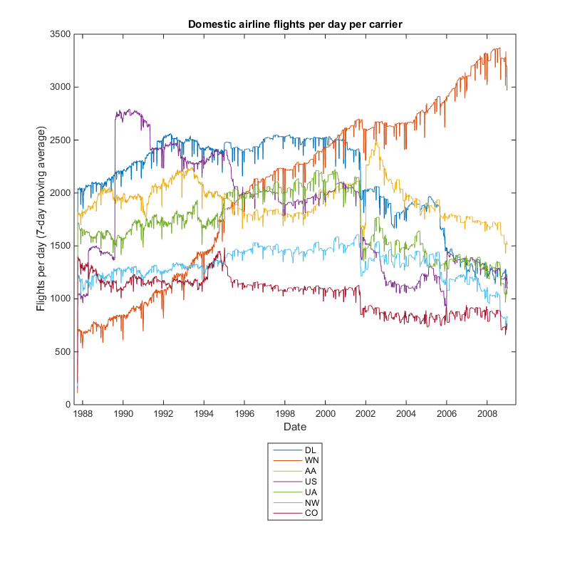
The interesting characteristic highlighted by the plot is the growth of Southwest Airlines (WN) during this time period.
Running mapreduce on Hadoop
The code we have just created was done so on our desktop computer and it allows us to analyze data that normally would not fit into the memory of our machine. But what if our data was stored on the "big data" platform, Hadoop® and the data set is too large to reasonably transfer to our desktop computer?
Using Parallel Computing Toolbox along with MATLAB® Distributed Computing Server™, this same code can be run on a remote Hadoop cluster. The map and reduce functions would remain unchanged, but two configuration changes are required:
- Our datastore is updated to reference the location of the data files in the Hadoop® Distributed File System (HDFS™).
- The mapreducer object is updated to reference Hadoop as the runtime environment.
After these configuration changes, the algorithm can then be run on Hadoop.
MATLAB Compiler can be used to deploy applications created using MapReduce, and it can also generate Hadoop specific components for use in production settings.
Conclusion
Learn more about MapReduce in MATLAB with our algorithm examples and let us know how you might see MapReduce being used to analyze your big data here.


コメント
コメントを残すには、ここ をクリックして MathWorks アカウントにサインインするか新しい MathWorks アカウントを作成します。