Visualizing Facebook Networks with MATLAB
When one of my guest bloggers, Toshi posted, Can We Predict a Breakup? Social Network Analysis with MATLAB, he got several questions about the new graph and network algorithms capabilities in MATLAB introduced in R2015b. He would like to do a follow-up post to address some of those questions.
Contents
Questions from the Readers
In the comment section of my recent post about social network analysis, QC asked if there was any way to plot very large scale network (>10000 nodes) with uniform degree, and Christine Tobler kindly provided an example and a link to a dataset collection. I would like to build on her comment in this post.
Plotting Large Scale Network in MATLAB
Can MATLAB plot large scale network with more than 10,000 nodes? Let's start by reproducing Christine's example that plots a graph with 10,443 nodes and 20,650 edges, representing an L-shaped grid.
n = 120;
A = delsq(numgrid('L',n));
G = graph(A,'OmitSelfLoops');
plot(G)
title('A graph with 10,443 nodes and 20,650 edges')

Facebook Ego Network Dataset
For datasets, Christine suggested the Stanford Large Network Dataset Collection. I decided to take her up on her suggestion using its Facebook dataset. This dataset contains anonymized personal networks of connections between friends of survey participants. Such personal networks represent friendships of a focal node, known as "ego" node, and such networks are therefore called "ego" networks.
Let's download "facebook.tar.gz" and extract its content into a "facebook" directory in the current folder. Each file starts with a node id and ends with suffix like ".circle", or ".edges". Those are ids of the "ego" nodes. We can run loadFBdata.m to load data from those files. I will just reload the preprocessed data.
clearvars                                           % clear workspace
% loadFBdata                                        % run script
load facebook                                       % or load mat file
who
Your variables are:

circles    egofeat    feat       graphs
edges      egoids     featnames
Visualize Combined Ego Networks
Let's first combine all 10 ego networks into a graph and visualize them in a single plot. This combined network has a little fewer than 4,000 nodes but with over 84,000 edges. It also includes some ego nodes, which means those survey participants were not entirely unrelated to one another.
comb = vertcat(edges{:});                           % combine edges
comb = sort(comb, 2);                               % sort edge order
comb = unique(comb,'rows');                         % remove duplicates
comb = comb + 1;                                    % convert to 1-indexing
combG = graph(comb(:,1),comb(:,2));                 % create undirected graph
notConnected = find(degree(combG) == 0);            % find unconnected nodes
combG = rmnode(combG, notConnected);                % remove them

edgeC = [.7 .7 .7];                                 % gray color

figure
H = plot(combG,'MarkerSize',1,'EdgeColor',edgeC, ...% plot graph
    'EdgeAlpha',0.3);
title('Combined Ego Networks')                      % add title
text(17,13,sprintf('Total %d nodes', ...            % add node metric
    numnodes(combG)))
text(17,12,sprintf('Total %d edges', ...            % add edge metric
    numedges(combG)))
text(17,11,'Ego nodes shown in red')                % add edge metric

egos = intersect(egoids + 1, unique(comb));         % find egos in the graph
highlight(H,egos,'NodeColor','r','MarkerSize',3)    % highlight them in red
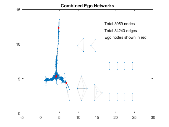
Visualize a Single Ego Network - Degree Centrality
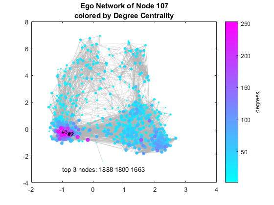
One of the most basic analyses you can perform on a network is link analysis. Let's figure out who are the most well connected in this graph. To make it easy to see, we can change the color by number of connections, also known as degree, and therefore this is a metric known as degree centrality. The top 3 nodes by degree are highlighted in the plot and they all belong to the same cluster. They are very closely connected friends!
Please note that the ego node is not included in this analysis as readme-Ego.txt says:
The 'ego' node does not appear (in the edge list), but it is assumed
that they follow every node id that appears in this file.
By nature the ego node will always be the top node, so there is no point including it.
idx = 2;                                            % pick an ego node
egonode = num2str(egoids(idx));                     % ego node name as string
G = graphs{idx};                                    % get its graph
deg = degree(G);                                    % get node degrees
notConnected = find(deg < 2);                       % weakly connected nodes
deg(notConnected) = [];                             % drop them from deg
G = rmnode(G, notConnected);                        % drop them from graph
[~, ranking] = sort(deg,'descend');                 % get ranking by degree
top3 = G.Nodes.Name(ranking(1:3));                  % get top 3 node names

figure
colormap cool                                       % set color map
H = plot(G,'MarkerSize',log(deg), ...               % node size in log scale
    'NodeCData',deg,...                             % node color by degree
    'EdgeColor',edgeC,'EdgeAlpha',0.3);
labelnode(H,top3,{'#1','#2','#3'});                 % label top 3 nodes
title({sprintf('Ego Network of Node %d', ...        % add title
    egoids(idx)); 'colored by Degree Centrality'})
text(-1,-3,['top 3 nodes: ',strjoin(top3)])         % annotate
H = colorbar;                                       % add colorbar
ylabel(H, 'degrees')                                % add metric as ylabel
Ego Network Degree Distribution
Let's check out the histogram of degrees between the ego network we just looked and the combined ego networks. People active on Facebook will have more edges than those not, but a few people have a large number of degrees and the majority have small number of degrees, and difference is large and looks exponential.
figure
histogram(degree(combG))                            % plot histogram
hold on                                             % don't overwrite
histogram(degree(G))                                % overlay histogram
hold off                                            % restore default
xlabel('Degrees')                                   % add x axis label
ylabel('Number of Nodes')                           % add y axis label
title('Degree Distribution')                        % add title
legend('The Combined Ego Networks', ...             % add legend
    sprintf('Ego Network of Node %d',egoids(idx)))
text(150,700,'Median Degrees')                      % annotate
text(160,650,sprintf('* Node %d: %d', ...           % annotate
    egoids(idx),median(degree(G))));
text(160,600,sprintf('* Combo    : %d', ...         % annotate
    median(degree(combG))));
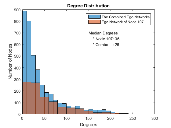
You'll notice that median degrees seem a bit small. That's because those are from nodes included in ego networks that contain nodes that are connected to ego nodes only. So we don't see other nodes that are not connected to the ego nodes (friends of friends). If you count the number of nodes in each ego network, you can see the degrees of each ego node, because ego nodes are supposed to be connected to all other nodes in their respective ego networks. The median is now 1404. Is this larger or smaller than the number of your Facebook friends?
deg = cellfun(@(x) numnodes(x), graphs);            % degrees of all graphs
median_deg = median(deg)                            % median degrees
median_deg =
        1404
Shortest Paths
We looked at degrees as a metric to evaluate nodes, and it makes sense - the more friends a node has, the better connected it is. Another common metric is shortest paths. While degrees measure direct connections only, shortest paths consider how many hops at mininum you need to make to traverse from one node to another. Let's look at an example of the shortest path between the top node 1888 and another node 483.
[path, d] = shortestpath(G,top3{1},'483');          % get shortest path

figure
H = plot(G,'MarkerSize',1,'EdgeColor',edgeC);       % plot graph
highlight(H,path,'NodeColor','r', ...               % highlight path
    'MarkerSize',3,'EdgeColor','r','LineWidth',2)
labelnode(H,path, [{'Top node'} path(2:end)])       % label nodes
title('Shortest Path between Top Node and Node 483')% add title
text(1,-3,sprintf('Distance: %d hops',d))           % annotate
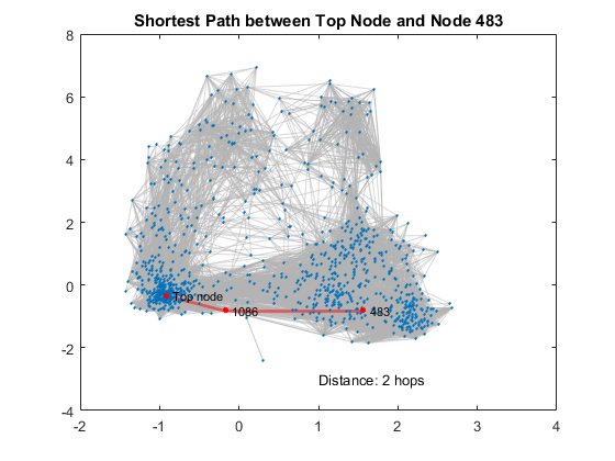
Closeness Centrality
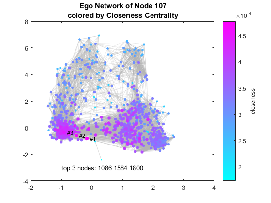
Distances measured by shortest paths can be used to compute closeness centrality, as defined in Wikipedia. Let's reload the pre-computed distances using the spdist function I wrote. Those with high closeness scores are the ones you want to start with when you want to spread news through your ego network.
load dist

closeness = 1./sum(dist);                           % compute closeness
[~, ranking] = sort(closeness, 'descend');          % get ranking by closeness
top3 = G.Nodes.Name(ranking(1:3));                  % get top 3 node names

figure
colormap cool                                       % set color map
H = plot(G,'MarkerSize',closeness*10000, ...        % node size by closeness
    'NodeCData',closeness,...                       % node color by closeness
    'EdgeColor',edgeC,'EdgeAlpha',0.3);
labelnode(H,top3,{'#1','#2','#3'});                 % label top 3 nodes
title({sprintf('Ego Network of Node %d', ...        % add title
    egoids(idx)); 'colored by Closeness Centrality'})
text(-1,-3,['top 3 nodes: ',strjoin(top3)])         % annotate
H = colorbar;                                       % add colorbar
ylabel(H, 'closeness')                              % add metric as ylabel
Can You Use Your Own Facebook Data?
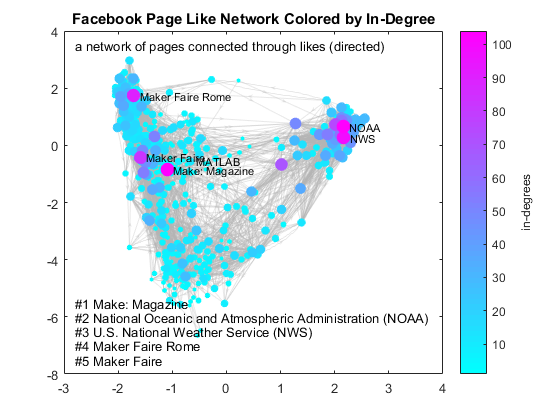
Hopefully this post has provided a sufficient basis for further exploration with the SNAP Collection dataset. You may also want to try this on your own data. Unfortunately, you can't analyze your own Facebook friends graph because Facebook discontinued this API service. You can, however, use apps like Netvizz to extract a "page like network", which represents Facebook pages connected through likes. Here is the plot that shows the network of Facebook pages connected to the MATLAB page through likes using a pre-computed graph. Because this is a directed graph, we will use in-degree as the metric. It means we only count when a page is liked by other pages, but not when it likes others.
load fbpagegraph                                    % reload data
deg = indegree(G);                                  % get in-degrees
[~,ranking] = sort(deg,'descend');                  % rank by in-degrees
top5 = G.Nodes.Name(ranking(1:5));                  % get top 5

figure
colormap cool                                       % set colormap to cool
H = plot(G,'MarkerSize',log(deg+2)*2, ...           % log scale node size by in-degree
    'NodeCData',deg, ...                            % color by in-degree
    'EdgeColor',edgeC,'EdgeAlpha', 0.3);
labelnode(H,'MATLAB','MATLAB')                      % highlight MATLAB
labelnode(H,top5,{'Make: Magazine','NOAA','NWS','Maker Faire Rome','Maker Faire'})
H = colorbar;                                       % add colorbar
ylabel(H, 'in-degrees')                             % add metric
title('Facebook Page Like Network Colored by In-Degree')
text(-2.8,3.5,'a network of pages connected through likes (directed)')
ann = {lab,top5};                                   % generate label
text(pos(:,1),pos(:,2),strcat(ann{:}))              % add annotations
Summary
We only scratched the surface with the SNAP Collection - just one ego network out of 10 for Facebook, and each comes with more anonymized meta data, such as eduction, hometown, etc. and you can figure out what binds those close-knit friends by analyzing common attributes. Furthermore, the SNAP Collection also includes datasets from other sources, sugh as Twitter and Google Plus. You can also use Netvizz to extract data on Facebook pages you liked. Play around with those datasets and let us know what you find!


댓글
댓글을 남기려면 링크 를 클릭하여 MathWorks 계정에 로그인하거나 계정을 새로 만드십시오.