Data Scaling for Scattered Interpolation
Today's guest blogger is Josh Meyer, a Technical Writer for the MATLAB Math and Big Data teams. He is going to discuss a common issue encountered in scattered data interpolation, and how to fix it!
Contents
The Problem
A common issue that can arise while performing interpolation on scattered data is that the resulting functional surface seems to be of lower quality than you would expect. For example, when the surface does not seem to pass through all of the sample data points. This post explores how and why the scaling of scattered data can affect the interpolation results.
Let's jump right into an example so you can see what I'm talking about. Imagine you just collected data from sensors to sample some values at several points. Ultimately you want to fit a surface to the data so that you can approximate the value of the underlying function at points where you don't have data. So, you start by plotting.
rng default
x = rand(500,1)/100;
y = 2.*(rand(500,1)-0.5).*90;
vals = (x.*100).^2;

ptColor = [.6 .07 .07];
plot3(x,y,vals,'.','Color',ptColor)
grid
xlabel('x')
ylabel('y')
zlabel('v(x,y)')
title('Scattered Data Points')
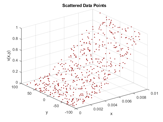
Next, you use scatteredInterpolant to create an interpolant for the data. This computes an interpolating function for the observed points, allowing you to query the function anywhere within its convex hull. You create a grid of query points, evaluate the interpolant at those points, and plot the functional surface. All done!
F = scatteredInterpolant(x,y,vals);
X = linspace(min(x),max(x),25);
Y = linspace(min(y),max(y),25);
[xq, yq] = meshgrid(X,Y);
zq = F(xq,yq);
hold on
triColor = [0.68 0.88 0.95];
surf(xq,yq,zq,'FaceColor',triColor)
hold off
xlabel('x')
ylabel('y')
zlabel('v(x,y)')
title('Scattered Data with Interpolated Surface')
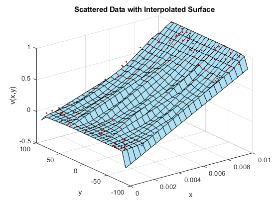
... but wait, the result is definitely not what you expected! What are all of those "folds" in the surface? And why does it look like the surface doesn't pass through all the points? Interpolated surfaces should pass through all of the data points!
Let's take a quick detour to talk about scattered data interpolation before coming back to this problematic data.
Background on Scattered Interpolation
Unlike gridded interpolation where the point locations are well-defined, scattered data presents different challenges. To find the interpolated value at a given query point, you need to use the values of nearby points. But how can you do that when the data is scattered around? The location of a point can't be used to predict the location of another point. And comparing the locations of all the points ad nauseum to determine which are close to a given query point is not a very efficient approach.
X = [-1.5  3.2; 1.8  3.3; -3.7  1.5;
    -1.5  1.3; 0.8  1.2; 3.3  1.5;
    -4.0 -1.0; -2.3 -0.7; 0   -0.5;
    2.0 -1.5;  3.7 -0.8; -3.5 -2.9;
    -0.9 -3.9; 2.0 -3.5;  3.5 -2.25];
V = X(:,1).^2 + X(:,2).^2;
plot(X(:,1),X(:,2),'r*')
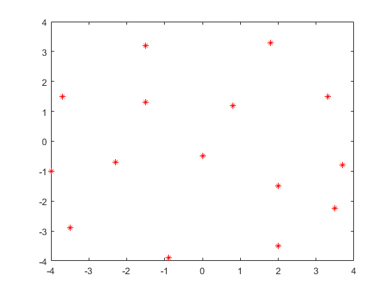
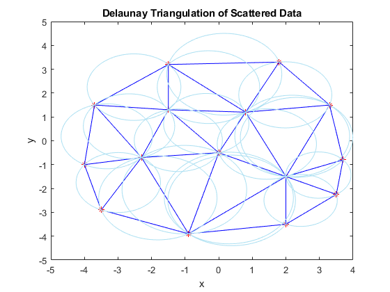
To solve this, MATLAB first computes a Delaunay triangulation of the scattered data. This creates a series of triangles out of the data points, such that the circumscribed circles created by the vertices of each triangle do not enclose any points. The computed Delaunay triangulation is unique, up to trivial symmetries. And the best part is, the triangulation can be easily queried to determine what points are closest to a given query point.
This plot shows the Delaunay triangulation and the circumscribed circles for the scattered data. Notice that the red data points lie on the boundaries of one or more circumscribed circles, but none of them lie in the interior of one of the circles.
tr = delaunayTriangulation(X(:,1),X(:,2));
[C,r] = circumcenter(tr);
a = C(:,1);
b = C(:,2);
pos = [a-r, b-r, 2*r, 2*r];
hold on
triplot(tr)
for k = 1:length(r)
    rectangle('Position',pos(k,:),'Curvature',[1 1],'EdgeColor',triColor)
end
xlabel('x')
ylabel('y')
title('Delaunay Triangulation of Scattered Data')
hold off
Armed with the triangulation of the data, finding the value of the interpolated surface at a given query point becomes a problem of querying the triangulation structure to determine which triangle encloses the query point. Then, the data points comprising the vertices of that triangle can be used to calculate the value of the interpolated surface at the query point, depending on which interpolation method is being used (nearest-neighbor, linear, etc...).
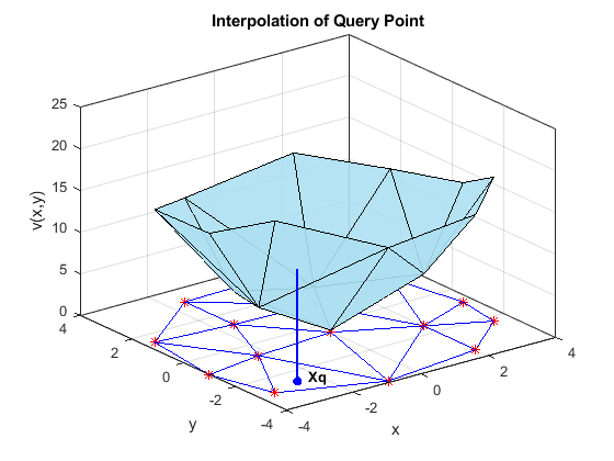
This plot shows a query point in a 2-D triangulation. To find the interpolated value at this query point, MATLAB uses the vertices of the enclosing triangle. By repeating this calculation at many different query points, a functional surface for the data forms. This functional surface allows you to make predictions at points where you did not collect data.
triplot(tr)
hold on
plot(X(:,1),X(:,2),'r*')
trisurf(tr.ConnectivityList,X(:,1),X(:,2),V,...
    'FaceColor',triColor, ...
    'FaceAlpha',0.9)
axis([-4, 4, -4, 4, 0, 25]);
grid on
plot3(-2.6,-2.6,0,'*b','LineWidth', 1.6)
plot3([-2.6 -2.6]',[-2.6 -2.6]',[0 13.52]','-b','LineWidth',1.6)
hold off
view(322.5, 30);
text(-2.0, -2.6,'Xq',...
    'FontWeight','bold', ...
    'HorizontalAlignment','center',...
    'BackgroundColor','none');
xlabel('x')
ylabel('y')
zlabel('v(x,y)')
title('Interpolation of Query Point')
Back to the Problem
Now that we know scatteredInterpolant uses a Delaunay triangulation of the data to perform its calculations, let's examine the underlying triangulation of the data we are having trouble interpolating.
tri = delaunayTriangulation(x,y);
triplot(tri)
hold on
plot(x,y,'r*')
hold off
xlabel('x')
ylabel('y')
title('Triangulation of Original Data')
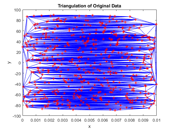
What a mess! There are only a few small pockets of reasonable triangles, with most of them being long and thin, connecting points that are far away from each other. It looks like the triangulation does pass through all of the data points, while the poor interpolated surface we saw earlier does not. We would expect that interpolated surface to look better.
Based on this triangulation, MATLAB has the not-enviable job of determining which of those long, thin triangles each query point lies in. And this brings us to ...
Cause of the Problem
The poor interpolation results are caused by the very different scales of the data (the x-axis ranges from [0, 0.01] and the y-axis from [-100, 100]) and the resulting long, thin triangles in the triangulation. After MATLAB classifies the query points into their corresponding triangles, it then uses the triangle vertices to find the value of the interpolated surface. Since the long, thin triangles have vertices that are far away from each other, this results in the local values of the interpolated surface being based on the values of far away points, rather than neighboring points.
Here is a GIF showing what happens to a triangulation as the x-data is scaled, while the y-data is constant. What starts out as a well-defined triangulation quickly becomes full of many long, thin triangles.

The data is effectively being shoved into a smaller and smaller area along the x-axis. If the axes are kept equal, the above animation looks like this.

Clearly, the triangulation underpinning the scattered interpolation calculation is sensitive to distortions in the data. The algorithm expects the x,y-coordinates to be reasonably scaled relative to each other. But, why?
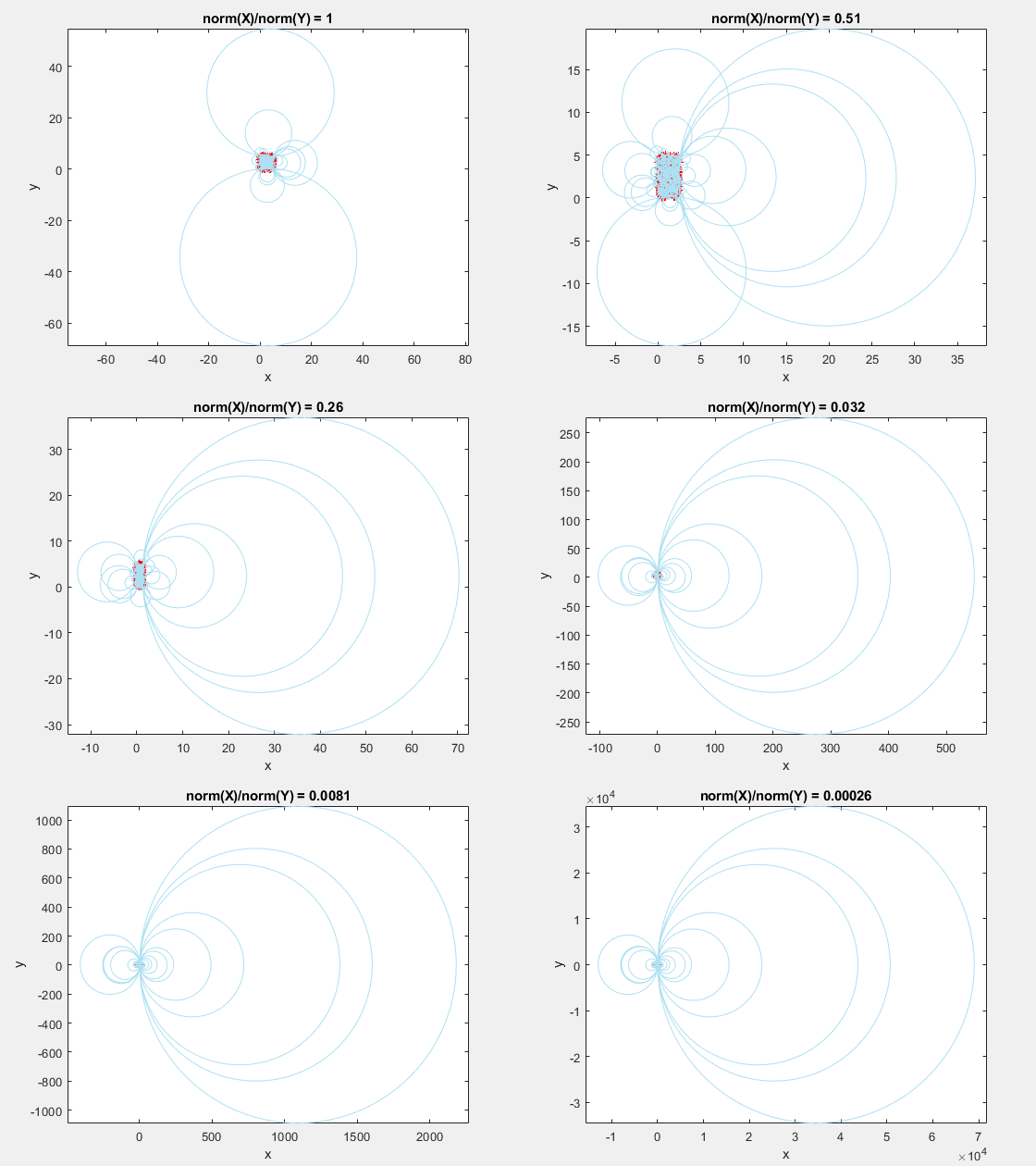
This behavior stems from the use of circumscribed circles in the Delaunay triangulation algorithm. When you squeeze the data in one direction, you are effectively altering the radii of the circumscribed circles. Taken to the extreme, as the points get squeezed together and become a straight line in one dimension, the radii of the circumscribed circles goes to infinity since the locus of points equidistant from the center of the circle becomes a straight line. The distribution of triangles is increasingly due to the proximity of the points in the y direction, hence why points that have close y values but very different x values become the triangle vertices.
If we add the circumscribed circles to the above animation, you can see that the radius of the circles blows up as the data gets squeezed.
Normalization to the Rescue
The solution to this issue is typically to remove the distortions in the data by normalizing. Normalization can improve the interpolation results in some cases when the triangulation has many thin triangles, but in others it can compromise the accuracy of the solution. Whether to use normalization is a judgment made based on the nature of the data being interpolated.
- Benefits: Normalizing your data can potentially improve the interpolation result when the independent variables have different units and substantially different scales. In this case, scaling the inputs to have similar magnitudes might improve the numerical aspects of the interpolation. An example where normalization would be beneficial is if x represents engine speed in RPMs from 500 to 3500, and y represents engine load from 0 to 1. The scales of x and y differ by a few orders of magnitude, and they have different units.
- Cautions: Use caution when normalizing your data if the independent variables have the same units, even if the scales of the variables are different. With data of the same units, normalization distorts the solution by adding a directional bias, which affects the underlying triangulation and ultimately compromises the accuracy of the interpolation. An example where normalization is erroneous is if both x and y represent locations and have units of meters. Scaling x and y unequally is not recommended because 10 m due East should be spatially the same as 10 m due North.
For our problem, let's assume x and y have different units and normalize them so that they have similar magnitudes. You can use the relatively new normalize function to do this; by default it uses Z-scores of the data. This transforms the data so that the original mean $\mu$ becomes 0, and the original standard deviation $\sigma$ becomes 1:
$$x' = \frac{\left(x - \mu\right)}{\sigma}.$$
This normalization is very common and is also called standardization.
x = normalize(x);
y = normalize(y);
Now that the data is normalized, let's take a look at the triangulation.
tri = delaunayTriangulation(x,y);
triplot(tri)
hold on
plot(x,y,'r*')
hold off
xlabel('x')
ylabel('y')
title('Triangulation of Normalized Data')
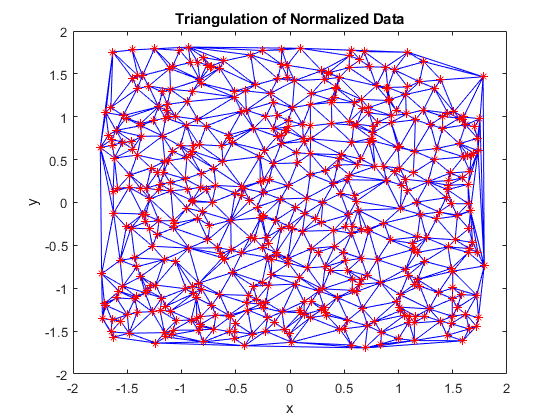
This is much better! The triangles are mostly well defined. There are only a few pockets of long, thin triangles near the edges. Let's take a look at the scattered interpolation surface now.
X = linspace(min(x),max(x),25);
Y = linspace(min(y),max(y),25);
[xq, yq] = meshgrid(X,Y);
F = scatteredInterpolant(x,y,vals);
zq = F(xq,yq);
plot3(x,y,vals,'.','Color',ptColor)
hold on
surf(xq,yq,zq,'FaceColor',triColor)
hold off
grid on
xlabel('x')
ylabel('y')
zlabel('v(x,y)')
title('Normalized Data with Interpolated Surface')
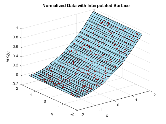
In this case, normalizing the sample points permits scatteredInterpolant to compute a better triangulation, and thus a better interpolated surface.
Data Scaling
Normalization is just one form of data scaling. With normalization you are changing the shape of the distribution of data and shifting the location of the mean value.

You can also rescale the data, changing the extent of its largest and smallest values (for example, making 0 the smallest value and 1 the largest value). When you rescale data you preserve the shape of the distribution but squeeze or expand it along the number line. This changes the mean value but preserves the standard deviation.

Data scaling is important to pay attention to. If the data is not properly scaled, it can hide relationships in the data or distort their strength. The results of some algorithms can vary a lot depending on the exact scaling used. We just saw how the triangulation of scattered data is sensitive to scaling, but it can cause problems in other algorithms as well. For example, machine learning algorithms typically depend on the Euclidean distance between points, so they are sensitive to the scaling of the data. Without proper scaling, some features will have too large a contribution compared to others, skewing the results.
But this is a broad topic best covered in another post!
Now let's extrapolate!
Do you use scattered data interpolation regularly in your work? If so tell us about it in the comments!
Acknowledgements
I'd like to thank Cosmin Ionita, Damian Sheehy, and Konstantin Kovalev for their valuable insights while I was writing this post.




댓글
댓글을 남기려면 링크 를 클릭하여 MathWorks 계정에 로그인하거나 계정을 새로 만드십시오.