
Solver Choice for Simulink and Simscape
Introduction
This blog post intends to provide best practices for choosing solvers in Simulink and Simscape. Gratitude goes to Tom Egel and Erin McGarrity whose materials are the foundation for anything written below. This article is certainly not aiming to replace the rock-solid documentation about solver choice, it is complementary and written for folks who:
- want to speed up simulations and increase accuracy,
- need a better understanding of the numerics involved.
This article will firstly talk about solver classification and naming, and secondly mention practical aspects about finding the optimal solver for your application and working around common mistakes. Simscape will not (yet) be covered specifically. Feel encouraged to leave a note in the comments section at the bottom if you are particularly interested in troubleshooting Simscape models.
This introduction may trigger two kinds of reactions:
- “I want to know more!”
-> Find here a Solver Workshop on FileExchange which is a hands-on deep dive into solver know-how including example models, slides and exercises. - “I don’t want to invest time into solver choice!”
-> I suggest having a look into auto solver, a feature that was added in release 2015a. It will choose an appropriate solver for your model automatically.
Motivation
This example of a Foucault pendulum (Link -> foucaultPendulum.slx) illustrates why solver choice is key! Depending on the solver choice ode45 (default) or ode23t, results of the pendulum displacements will be entirely different. As can be seen in the plots, ode23t leads to more meaningful results since the displacements should be symmetric. Sometimes, errors won’t be as obvious. My PhD supervisor typically said when discussing modeling strategies “Christoph, all models are wrong, but some of them are useful.” In the following, let’s try to make sure that simulation results will be useful.

Open and run the model “foucaultPendulum.slx” in the solver workshop on FileExchange to experience the illustrated solver behavior. Before talking about model stiffness which lead to the significant result deviations in the example above, let’s do the groundwork first and see what Simulink / Simscape solvers there are and how they can be classified.
Solver Classification and Naming
Names and their Meaning
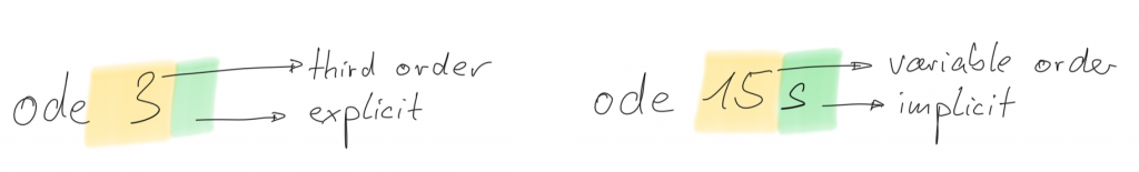
The most important info is carried by the solver names themselves. A single digit number represents a fixed-step solver, the number itself gives info about the order. Information on the integration scheme can also be obtained from the name. Solvers using an implicit scheme always come with an amended letter, explicit solvers only have the number. The amendment letters are abbreviations: “t” trapezoidal, “tb” trapezoidal-backward, “s” stiff and “x” extrapolation. If there is no amendment, that’s an explicit solver.
Classification
MathWorks solvers can be classified into 4 categories:
Step Size – Order – State Updates – Integration Scheme.
Step Size
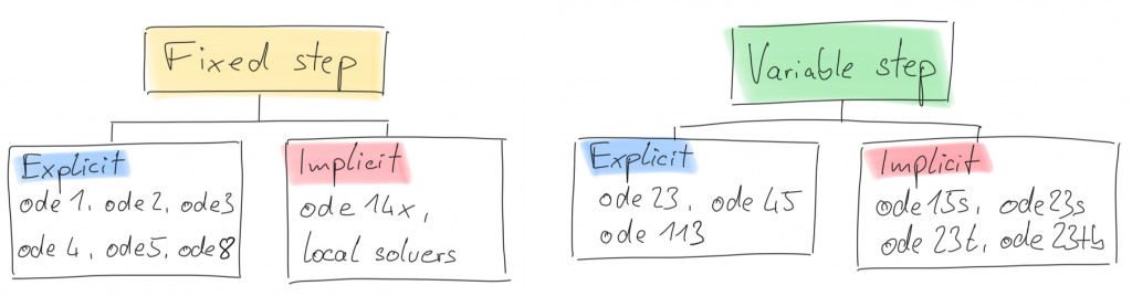
Fixed-step solvers are typically used for to meet accuracy requirements and are used when models will be deployed onto hardware such as microcontrollers (keyword: code generation). Variable step solvers automatically change the time step to meet requirements. They are typically used for plant model development. A variable-step solver might shorten the simulation time of your model significantly.
This model shows how a variable-step solver can shorten simulation time for a multi-rate discrete model. The model generates outputs at two different rates: every 0.5 s and every 0.75 s. To capture both outputs, the fixed-step solver must take a time step every 0.25 s (the fundamental sample time for the model).
Order
As mentioned before, the numbers used in the solver name specify the solver order. Choice of order has an impact on accuracy. Most often, a high-order solver is more efficient than a low-order solver. Variable-order solvers use multiple orders to solve the system of equations. For example, the implicit, variable-step ode15s solver uses first-order through fifth-order equations while the explicit, variable-step ode113 solver uses first-order through thirteenth-order. Solver’s step size and integration order have a huge impact on accuracy. In my mind, the simplest way of explaining is the following:
- Smaller step size and higher solver order both increase accuracy
- More accuracy is slower (at least for a fixed-step solver)
State Updates: Discrete vs. Continuous
Discrete and continuous solvers rely on the model blocks to compute the values of any discrete states. Blocks that define discrete states are responsible for computing the values of those states at each time step. However, unlike discrete solvers, continuous solvers use numerical integration to compute the continuous states that the blocks define.
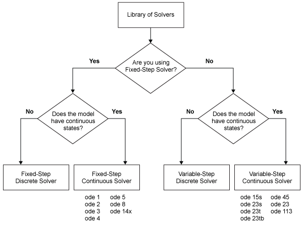
If your model has no continuous states, then Simulink switches to either the fixed-step discrete solver or the variable-step discrete solver. If your model has only continuous states or a mix of continuous and discrete states, choose a continuous solver from the remaining solver choices based on the dynamics of your model. Otherwise, an error occurs.
Integration Scheme: Explicit vs. Implicit
Explicit solvers use past information in the equations to compute next step. This is computationally simple but unstable as the system equations won’t be solved completely at any time. Instability is not necessary a problem because everything will be fine if the approximated solution is still within your desired margin of error. Implicit Solvers compute next steps self-consistently which is more computational work per step.
While you can apply an implicit or explicit continuous solver to solve all these systems, implicit solvers are designed specifically for solving stiff problems. Explicit solvers solve non-stiff problems. An ordinary differential equation problem is said to be stiff if the desired solution varies slowly, but there are closer solutions that vary rapidly. In short, one could say: a stiff system has both slowly and quickly varying continuous dynamics. The numerical method must then take small time steps to solve the system. Stiffness is an efficiency issue. The more stiff a system, the longer it takes to for the explicit solver to perform a computation. For example, most of the physical models built using the Simscape product family end up being stiff systems, in which case you would want to make sure you choose between stiff solvers.
Practical Aspects
Solver Choice
When you build and simulate a model, you can choose either type of solver based on the dynamics of the model. A model that contains several switches, like an inverter power system, needs a fixed-step solver. A variable-step solver is better suited for purely continuous models, like the dynamics of a mass spring damper system.
When you deploy a model as generated code, you can use only a fixed-step solver. If you selected a variable-step solver during simulation, use it to calculate the step size required for the fixed-step solver that you need at deployment.
Zero-Crossings
Note: This is relevant if you have chosen a variable step solver only.
A variable-step solver dynamically adjusts the time step size, causing it to increase when a variable is changing slowly and to decrease when the variable changes rapidly. Thus, the solver takes many small steps near a discontinuity, e.g. a zero-crossing. Zero crossing events may be sign changes or hard stops. Overall, this behavior improves accuracy but can lead to excessive simulation times.
Knowing that zero-crossing may slow your model down is already a major part of the solution. Find here a list of possible remedies:
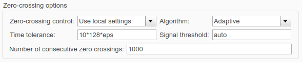
- Adjust the zero-crossing options
(Configuration parameters -> Additional options)- Increase number of consecutive zero crossings
- Switch to the adaptive algorithm
- Relax signal threshold
- Disable detection for specific blocks, see documentation
- Modify the model and reduce constraints
This is not just a setting, let me refer you to the solver workshop (FEX) for a hands-on example.
Algebraic Loops
An algebraic loop generally occurs when an input port with direct feedthrough is driven by the output of the same block, either directly, or by a feedback path through other blocks with direct feedthrough. Thus, the solver is forced to use iterative methods which is slow (!).
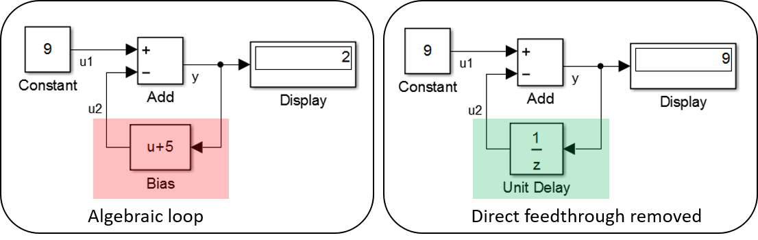
The best remedy is to avoid algebraic loops if possible, find a chapter helping you in the documentation or have a look at the solver workshop (FEX) introduced before.
This article is by no means complete nor is it the only publication about this topic. Same as for models that should be useful, I hope this text helps you in your daily work with Simulink. Feel encouraged to comment and suggest improvements or clarification.
Cheers Christoph
- Category:
- Automotive,
- Robotics,
- Simscape,
- Simulink,
- Workflow


Comments
To leave a comment, please click here to sign in to your MathWorks Account or create a new one.