Earlier in this series I have discussed the problem of plateaus. Specifically, how do you assign a flow direction to a DEM pixel that has no downhill neighbors? I proposed in part 5 that the problem could be addressed by using the interpolation technique in roifill to modify plateau values so that they are no longer equal, and then recomputing the flow direction based on the modified values.

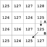
OK, true confessions time—I could never get this idea to really work! Here's a small set of DEM values to illustrate the typical problem:

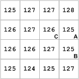
The pixels labeled A and B in the right column have no downhill neighbors. Modifying those values using roifill so they were no longer flat had the effect of raising pixel A above the value of pixel C. As a result, my recomputed flow directions had the amusing property that pixel C flowed to pixel A, and pixel A flowed to pixel C!

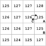
I discovered this problem while trying to understand why, in some cases, I was getting flow matrices that were singular.

So it was back to the drawing board. I eventually found a good solution in F. Meyer, "Skeletons and Perceptual Graphs," Signal Processing 16 (1989) 335-363. This paper has a couple of algorithms for determining ordering relationships among pixels on a plateau. One of the algorithms, called arrowing, turned to be suitable for computing flow matrix weights for plateau pixels. (Meyer credits Maisonneuve for the original idea.)

First scan. During the first scan every pair of neighbors (x,y) is considered. If the pixel x is higher than the pixel y, it is given an arrow towards y. During this scan all descending borders of all plateaus receive arrows.

Next scans. Until convergence, the following operation is repeated: if x and y are two neighbours sharing the same altitude, and if x possesses an arrow but not y, then y is given an arrow pointing towards x.

–pages 360-361

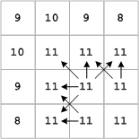
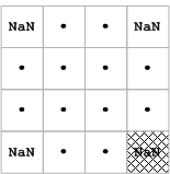
Here's an example showing how to compute flow directions using arrowing. Below, on the left, is a 4-by-4 matrix of DEM pixels. Some of these DEM pixels have no downhill neighbors. These pixels are indicated via NaNs in the matrix on the right.

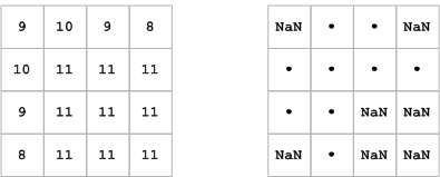
With our earlier method for calculating flow directions, the descending borders of plateaus already have flow directions computed for them, which means we can skip the first scan step of the arrowing algorithm. In each subsequent scan, we identify the pixels that do not have a flow direction yet, and which have equal-altitude neighbors that do. Here is the first set of such pixels:

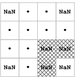
We'll say that each shaded pixel flows equally to all of its equal-altitude neighbors that already have flow directions established, like this:

On the second scan, we find only one pixel without a flow direction, and which has equal-altitude neighbors that do have flow directions:

And so we assign flow directions like this:

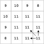
The third scan finds no pixels satisfying the criteria, so we know we're done.

Revisiting the example I started with, here's how the arrowing procedure assigns flow directions to pixels A and B:

The MATLAB code is a little too involved to show in detail here. If you care to see exactly how it works, look at the plateau_flow_weights subfunction of flow_matrix.m in my upslope area code on the MATLAB Central File Exchange.