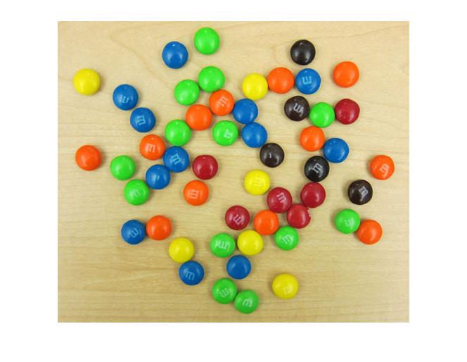
Last week I showed this picture of M&Ms on my desk, and I used it to raise some vague questions about the definition of the color green. Today I'll use this picture as an opportunity to demonstrate how to construct and visualize a two-dimensional histogram.

url = 'https://blogs.mathworks.com/images/steve/2010/mms.jpg';
rgb = imread(url);
imshow(rgb)

As a preparatory step, I'll first convert the pixels from the sRGB color space to the L*a*b* color space. I've written about the L*a*b* color before (09-May-2006, 19-Jun-2006). It does a couple of nice things. First, it separates perceived brightness (L*) from color (a* and b*). Second, as a rough approximation it is perceptually uniform. That is, Euclidean distances in the L*a*b* space correspond roughly uniformly to perceived color differences.

Here's how to do the conversion:

lab = applycform(rgb, makecform('srgb2lab'));

But I must note here that the values in lab aren't the normal mathematical quantities L*, a*, and b*. That's because those real values have been encoded (scaled, shifted, and quantized) to fit into unsigned 8-bit integers. So I'll use the function lab2double to convert these encoded values into the normal mathematical values.

lab = lab2double(lab);
a = lab(:,:,2);
b = lab(:,:,3);

I claimed above that the color information is in the a* and b* dimensions. Can we look at the a* and b* values in a way that lets us start to see the different M&M colors in the original image? I want to do it by constructing a two-dimensional histogram of the a* and b* values.

There are many different ways you could formulate and implement this in MATLAB. I've picked a method based on the functions interp1 and accumarray. The basic idea is to convert each a* value into a horizontal array subscript, convert each b* value into a vertical array subscript, and then use accumarray to accumulate values into a histogram.

First, let's set up a notion of our histogram bins in the a* and b* dimensions. I'll specify 101 bins according to their centers.

N = 101;
bin_centers = linspace(-100, 100, N);

I want to map a* and b* values such that bin centers become subscript values. I found it easy to think about this process in terms of the function interp1, but others might do it differently. I'll use linear interpolation and extrapolate to handle a* and b* values that are completely outside the range of the bin centers.

subscripts = 1:N;
ai = interp1(bin_centers, subscripts, a, 'linear', 'extrap');
bi = interp1(bin_centers, subscripts, b, 'linear', 'extrap');

Now I need to round the subscript matrices, ai and bi, and I also need to make sure all the subscript values lie between 1 and N.

ai = round(ai);
bi = round(bi);

ai = max(min(ai, N), 1);
bi = max(min(bi, N), 1);

Next we let accumarray do the heavy lifting of counting how many times each pair of subscript values occurs.

H = accumarray([bi(:), ai(:)], 1, [N N]);

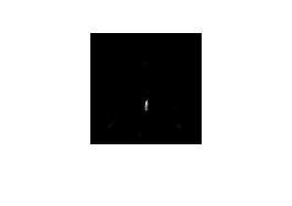
H is our two-dimensional histogram. Here's my first attempt at visualizing it. The second argument to imshow, [], tells imshow to autoscale the range values in H for display.

imshow(H, [])

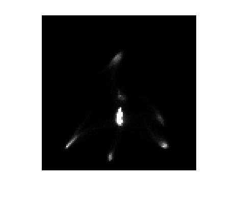
There are two issues I need to fix: the displayed image is a bit small, and the autoscaling didn't make the histogram detail very visible. Let's manually specify a different display scaling, and let's also ask imshow to display the image larger than normal.

figure
imshow(H, [0 1000], 'InitialMagnification', 300)

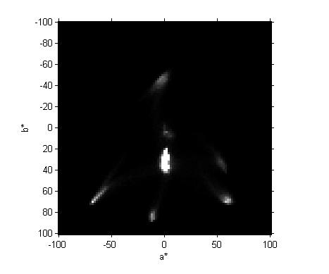
How about axes tickmarks and labels? Can we get the real a* and b* ranges to show up? Sure. We tell imshow the real horizontal coordinates corresponding to the left column and right column (the "xdata"), as well as the vertical coordinates corresponding to the top row and bottom row (the "ydata").

xdata = [min(bin_centers), max(bin_centers)];
ydata = xdata;
imshow(H,[0 1000], 'InitialMagnification', 300, 'XData', xdata, 'YData', ydata)

Oops, still no axes tickmarks and labels. That's because imshow doesn't display them by default. But we can manually turn them on with the axis function.

axis on
xlabel('a*')
ylabel('b*')

That's our completed two-dimensional histogram and visualization.

I think that next time I'll explore segmenting in the a*-b* plane. But as usual I'm making up these blog posts as I go along, so no promises.

Get the MATLAB code

Published with MATLAB® 7.11