More on segmenting in a*-b* space
I'm back to looking at M&Ms today. (Previous posts: 17-Dec-2010, 23-Dec-2010, 30-Dec-2010, 11-Jan-2011)
url = 'https://blogs.mathworks.com/images/steve/2010/mms.jpg';
rgb = imread(url);
imshow(rgb)
Last time I showed how I used imfreehand to segment the region in the a*-b* plane corresponding to the green M&Ms.

This time I'll use connected-components labeling and regionprops to segment the image based on all the colors, including the desk background.
I saved the previously computed a*-b* histogram in a MAT-file online; here's how to retrieve and display it.
matfile_url = 'https://blogs.mathworks.com/images/steve/2011/freehand_segment.mat';
temp_matfile = [tempname '.mat'];
urlwrite(matfile_url, temp_matfile);
s = load(temp_matfile);
delete(temp_matfile)
H = s.H;
imshow(H, [0 1000], 'InitialMagnification', 300, 'XData', [-100 100], ...
    'YData', [-100 100])
axis on
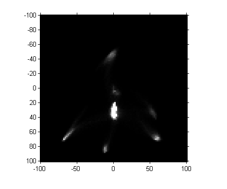
Next, let's threshold the image. (Magic Number Alert! I chose the threshold manually based on visual inspection of pixel values.)
mask = H > 100;
imshow(mask, 'InitialMagnification', 300, 'XData', [-100 100], ...
    'YData', [-100 100])
axis on
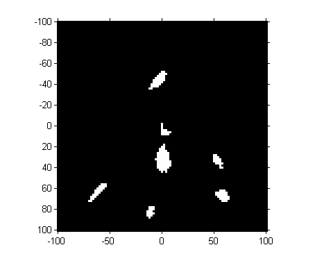
So we've got seven "blobs". Let's measure their centroids.
props = regionprops(mask, s.H, 'Centroid');
props(1)
ans =

    Centroid: [20.2143 82.5357]
centers = cat(1, props.Centroid)
centers =

   20.2143   82.5357
   45.4706   92.2353
   49.2973   29.0541
   51.6029   67.1765
   52.2667   53.4667
   77.8000   67.8000
   80.1724   84.4483
These centroid values are in the intrinsic pixel coordinates of the image. To convert them to a* and b* values, we have to scale and shift.
ab_centers = 2*centers - 102
ab_centers =

  -61.5714   63.0714
  -11.0588   82.4706
   -3.4054  -43.8919
    1.2059   32.3529
    2.5333    4.9333
   53.6000   33.6000
   58.3448   66.8966
a_centers = ab_centers(:,1);
b_centers = ab_centers(:,2);
Next question: where are these centers, and what are the regions in the a*-b* plane closest to each one? The voronoi function shows you both.
hold on
voronoi(a_centers, b_centers, 'r')
hold off
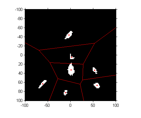
To perform a nearest-neighbor classification of all the pixels, let's compute the Delaunay triangulation, from which we can easily do the nearest-neighbor calculation.
dt = DelaunayTri(a_centers, b_centers)
dt =

  DelaunayTri

  Properties:
      Constraints: []
                X: [7x2 double]
    Triangulation: [7x3 double]
Compute the a* and b* values of all the pixels:
lab = lab2double(applycform(rgb, makecform('srgb2lab')));
L = lab(:,:,1);
a = lab(:,:,2);
b = lab(:,:,3);
For every pixel in the original image, find the closest a*-b* centroid by using the nearestNeighbor function with the Delaunay triangulation.
X = nearestNeighbor(dt, a(:), b(:));
X = reshape(X, size(a));
I would like to make a colormap of the seven colors in our segmentation. We have a* and b* values for each of the colors, but not L* values. We could just make up a constant L* value. Instead, I'll compute the mean L* value for all the pixels closest to the centroid of each of the histogram blobs.
L_mean = zeros(size(a_centers));
for k = 1:numel(L_mean)
    L_mean(k) = mean(L(X == k));
end
Now we convert the L*a*b* values corresponding to each of our seven colors back to RGB using applycform.
map = applycform([L_mean, a_centers, b_centers], makecform('lab2srgb'))
map =

    0.2587    0.8349    0.1934
    0.8724    0.8465    0.0271
    0.1095    0.4111    0.6803
    0.8382    0.7591    0.5286
    0.3304    0.2993    0.2751
    0.7264    0.2055    0.2008
    0.9653    0.3595    0.0690
And finally we can use X and map to display our segmented result as an indexed image.
close all
imshow(X, map)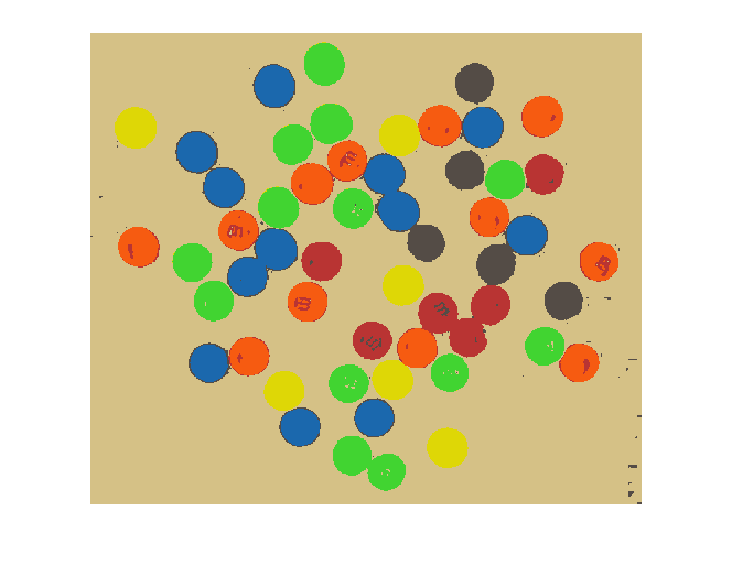
Not bad!
Unless I have some inspiration between now and next week, I might be ready to let this image go and search for something else to write about.




댓글
댓글을 남기려면 링크 를 클릭하여 MathWorks 계정에 로그인하거나 계정을 새로 만드십시오.