Homomorphic filtering – part 2
I'd like to welcome back guest blogger Spandan Tiwari for the second post in his two-part series on homomorphic filtering.
Last time we looked at how to apply a simple homomorphic filter. Today we continue our discussion on homomorphic filtering. First I'll load the variables I, H, and Ihmf that I computed last time.
load homomorphic_part1
In homomorphic filtering we apply a high-pass filter to the log-transformed image. The high-pass filtering step provides us with an opportunity to simultaneously apply other enhancements to the image. Consider a modified version of the high-pass filter $H(u,v)$ that we used last time.
$$ H_{e}(u,v) = \alpha + \beta \ H(u,v) $$
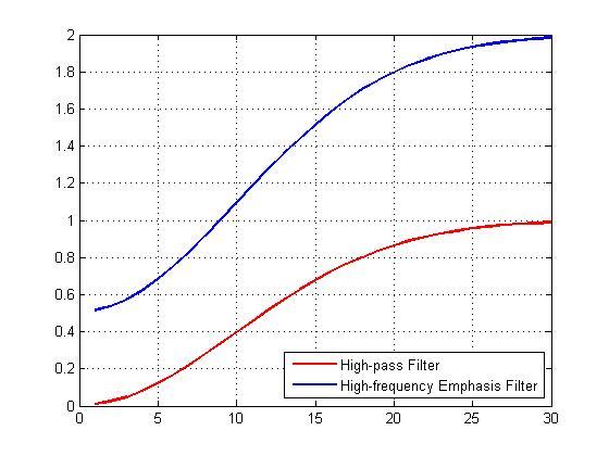
We added an offset and a scaling factor for the Gaussian high-pass filter. If $\alpha < 1$ and $\beta > 1$, this filter will amplify the high-frequency components more than the low-frequency components. This filter is called high-frequency emphasis filter. The resulting image, typically, is sharper and also has better contrast. We choose $\alpha = 0.5$ and $\beta = 1.5$, and formulate the high-frequency emphasis filter.
alpha = 0.5;
beta = 1.5;
Hemphasis = alpha + beta*H;
Let's compare the original high-pass filter and the high-frequency emphasis filter by looking at their cross-sections.
plot(1:30,H(1,1:30),'r',1:30,Hemphasis(1,1:30),'b','LineWidth',2);
grid on;
legend('High-pass Filter','High-frequency Emphasis Filter','Location','best');
Now let's apply the filter and look at the result of homomorphic filtering. The image below shows the original (on the left) and the homomorphic filtered (on the right) images together. If you compare the two images you can see that the gradual change in illumination in the left image has been corrected to a large extent in the image on the right.
If = fft2(I, M, N);
Iout = real(ifft2(Hemphasis.*If));
Iout = Iout(1:size(I,1),1:size(I,2));

Ihmf_2 = exp(Iout) - 1;

imshowpair(I, Ihmf_2, 'montage')
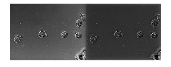
The non-uniform illumination has largely been corrected. Now let's compare our earlier result of homomorphic filtering with regular high-pass filter (below, left) and the result with high-frequency emphasis filter (below, right). We see that the latter seems to have better non-uniform illumination compensation of the two.
imshowpair(Ihmf, Ihmf_2, 'montage')
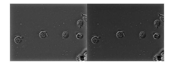
Also, looking at these two images side-by-side highlights an interesting effect. In the image on the left there seems to be a bright halo type artifact on the borders. This can be seen more clearly if we increase the contrast by applying histogram equalization on the image on the left using the histeq function. Note that I am normalizing the image using mat2gray before passing it to histeq.
imshow(histeq(mat2gray(Ihmf)))
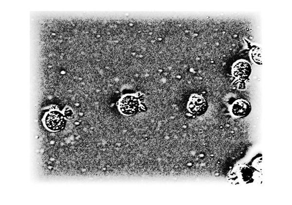
The halos on the borders can be seen clearly now. But if you look closely it is not just the image on the left that has the halo effect on the borders. The output from the high-frequency emphasis filter (image on the right) also has a similar, but less-pronounced, halo effect. Let's look at the histogram equalized version of both these images together to make this more apparent.
imshowpair(histeq(mat2gray(Ihmf)), histeq(mat2gray(Ihmf_2)), 'montage')
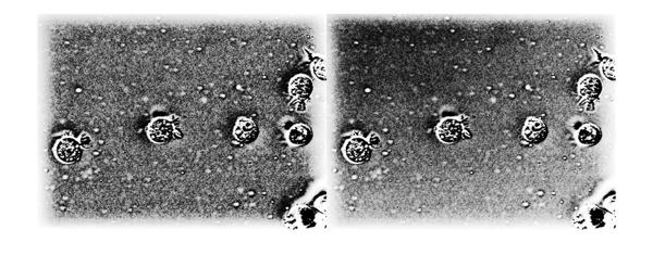
So why does this happen? Well, this artifact is because we padded the image with zeros during filtering, and the effect of the zeros leak into the image domain. A solution would be to apply a windowing function (such as the Hanning window) instead of zero-padding, before computing the Discrete Fourier Transform. But this solution is not appropriate in our situation because it is the same as introducing another slowly-varying multiplicative undesired signal, just like the non-uniform illumination signal that we are trying to remove. Another way to help the situation is to pad the image by replicating the intensity at the borders of the image instead of padding the image with zeros. Although this won't eliminate the artifacts due to leakage completely, it will mitigate their severity. To achieve the replicate style padding, we will have to pad the image ourselves, instead of letting fft2 pad it for us. We will use Image Processing Toolbox function padarray for this.
paddedI = padarray(I,ceil(size(I)/2)+1,'replicate');
paddedI = paddedI(1:end-1,1:end-1);
Let's look at the result with the replicate style padding. I will show the results only for the high-frequency emphasis filter. We apply the high-frequency emphasis filter to the padded image.
If = fft2(paddedI);
Iout = real(ifft2(Hemphasis.*If));
Note that we padded the image on both sides in each dimension. This is unlike fft2 which appends trailing zeros along each dimension. Consequently, the output will also be padded on both sides.
imshow(Iout)
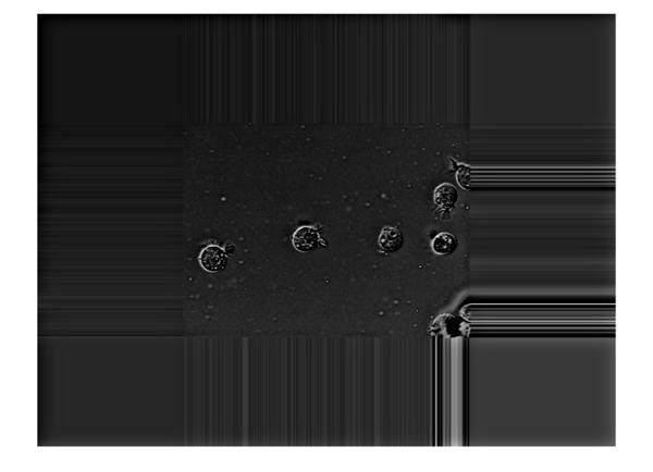
While cropping the image back to the original size we have to mindful of this and crop the image around the center of the larger output image.
Iout = Iout(ceil(M/2)-size(I,1)/2+1:ceil(M/2)+size(I,1)/2, ...
            ceil(N/2)-size(I,2)/2+1:ceil(N/2)+size(I,2)/2);
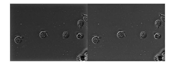
Let's apply the exponential and look at the result. The image on the left is the output with zero padding that we computed earlier. The one of the right is the output with replicate style padding. We can see that the halo effect has been mitigated to a large extent.
Ihmf_3 = exp(Iout) - 1;
imshowpair(Ihmf_2, Ihmf_3, 'montage')
Let's use histogram equalization to get a better a better look.
imshowpair(histeq(mat2gray(Ihmf_2)), histeq(mat2gray(Ihmf_3)), 'montage')
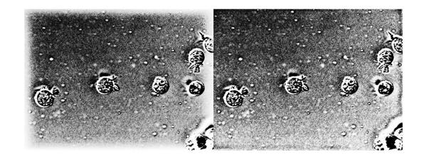
The halo effect at the border has been mitigated significantly. But we had to do some code mechanics to get homomorphic filtering to play well in the FFT-domain. This is where the spatial domain filtering might offer a better alternative. It is relatively simpler to do the replicate style padding in the spatial domain. Let's create a simple spatial domain high-pass filter. Although we can create a spatial kernel exactly equivalent to the frequency-domain Gaussian high-pass filter we used earlier, we won't get into that to keep things simple. Here we make a simple ideal high-pass filter.
filterRadius = sigma;
filterSize = 2*filterRadius + 1;
hLowpass = fspecial('average', filterSize);
hImpulse = zeros(filterSize);
hImpulse(filterRadius+1,filterRadius+1) = 1;
hHighpass = hImpulse - hLowpass;
Now we apply this high-pass filter in the spatial domain. To get the replicate style padding, we simply specify the 'replicate' option in imfilter. Then we apply the exponential to get the homomorphic filtered image.
Ihmf_spatial = imfilter(I, hHighpass, 'replicate');

Ihmf_spatial = exp(Ihmf_spatial) - 1;
Here's the filtered image (right) juxtaposed with the original input image (left).
imshowpair(I, Ihmf_spatial, 'montage')
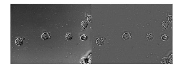
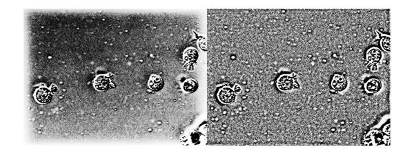
Again, we see that the non-uniform illumination has been corrected to a large extent and there aren't any noticeable border artifacts. To show the absence of the border artifacts let's look at the histogram equalized version of the output. For comparison we will also enhance the output from frequency-domain high-emphasis filtered image (with zero-padding), which is shown on the left. Again, we can see that there aren't any noticeable border artifacts after filtering in the spatial domain (image on the right).
imshowpair(histeq(mat2gray(Ihmf_2)), histeq(mat2gray(Ihmf_spatial)), 'montage');
Both frequency domain and spatial domain filtering offer some practical advantages of their own. Spatial domain filtering offers a straightforward way to get the padding right. Also, it might be faster for small kernel sizes. But the frequency domain offers an easier and more intuitive way to get the filter with desired frequency characteristics.
In conclusion, homomorphic filtering is a useful tool to have in your quiver of enhancement techniques. It may not be applicable as a generic enhancement technique, but it works well on a certain set of problems.
Which applications have you used homomorphic filtering for? Were there any specific problems you faced while using it? Let us know.
 Cleve’s Corner: Cleve Moler on Mathematics and Computing
 The MATLAB Blog
 Guy on Simulink
 MATLAB Community
 Artificial Intelligence
 Developer Zone
 Stuart’s MATLAB Videos
 Behind the Headlines
 File Exchange Pick of the Week
 Hans on IoT
 Student Lounge
 MATLAB ユーザーコミュニティー
 Startups, Accelerators, & Entrepreneurs
 Autonomous Systems
 Quantitative Finance
 MATLAB Graphics and App Building


Comments
To leave a comment, please click here to sign in to your MathWorks Account or create a new one.