Today I'll show you one way to visualize the sRGB color gamut in L*a*b* space with assistance with a couple of new functions introduced last fall in the R2014b release. (I originally planned to post this a few months ago, but I got sidetracked writing about colormaps.)

The first new function is called boundary, and it is in MATLAB. Given a set of 2-D or 3-D points, boundary computes, well, the boundary.

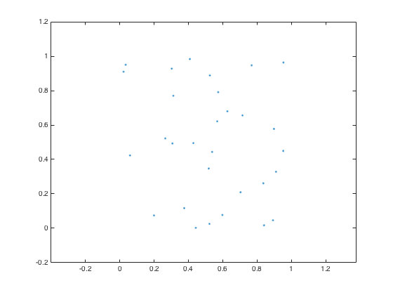
Here's an example to illustrate.

x = gallery('uniformdata',30,1,1);
y = gallery('uniformdata',30,1,10);
plot(x,y,'.')
axis([-0.2 1.2 -0.2 1.2])
axis equal

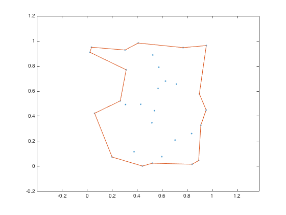
Now compute and plot the boundary around the points.

k = boundary(x,y);
hold on
plot(x(k),y(k))
hold off

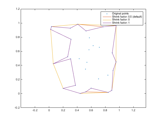
"But, Steve," some of you are saying, "that's not the only possible boundary around these points, right?"

Right. The function boundary has an optional shrink factor that you can specify. A shrink factor of 0 corresponds to the convex hull. A shrink factor of 1 gives a compact boundary that envelops all the points.

k0 = boundary(x,y,0);
k1 = boundary(x,y,1);
hold on
plot(x(k0),y(k0))
plot(x(k1),y(k1))
hold off
legend('Original points','Shrink factor: 0.5 (default)',...
    'Shrink factor: 0','Shrink factor: 1')

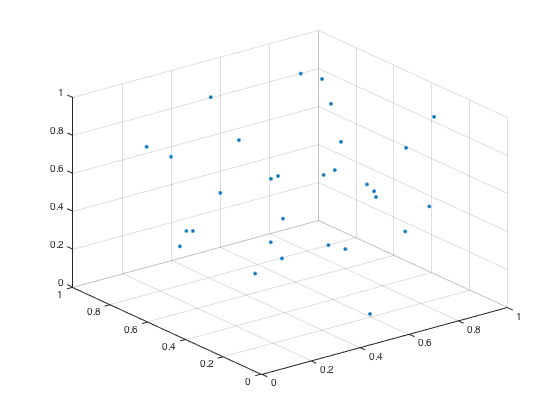
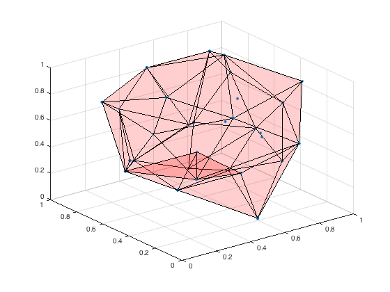
Here's a 3-D example using boundary. First, the points:

P = gallery('uniformdata',30,3,5);
plot3(P(:,1),P(:,2),P(:,3),'.','MarkerSize',10)
grid on

Now the boundary, plotted using trisurf:

k = boundary(P);
hold on
trisurf(k,P(:,1),P(:,2),P(:,3),'Facecolor','red','FaceAlpha',0.1)
hold off

The second new function I wanted to mention is rgb2lab. This function is in the Image Processing Toolbox. The toolbox could convert from sRGB to L*a*b* before, but this function makes it a bit easier. (And, if you're interested, it supports not only sRGB but also Adobe RGB 1998).

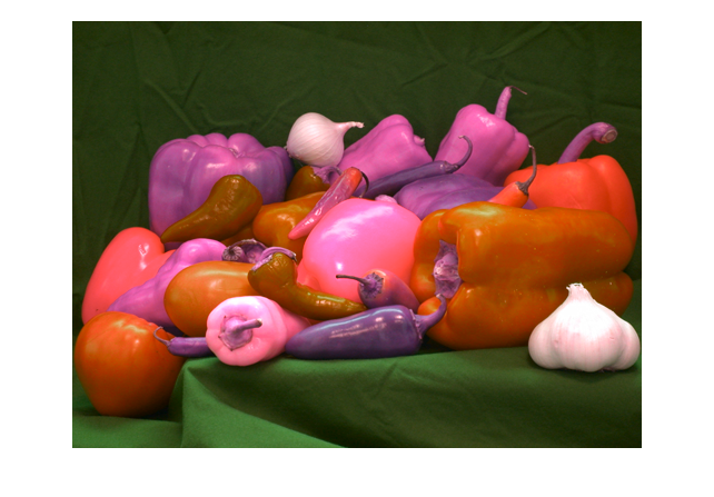
Just for grins, let's reverse the a* and b* color coordinates for an image.

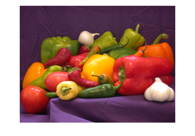
rgb = imread('peppers.png');
imshow(rgb)

lab = rgb2lab(rgb);
labp = lab(:,:,[1 3 2]);
rgbp = lab2rgb(labp);
imshow(rgbp)

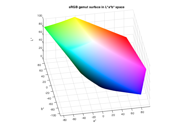
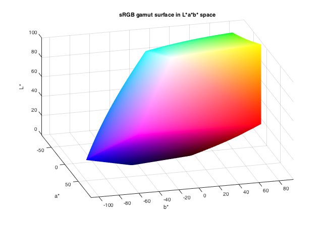
Now let's get to work on visualizing the sRGB gamut surface. The basic strategy is to make a grid of points in RGB space, transform them to L*a*b* space, and find the boundary. (We'll use the default shrink factor.)

[r,g,b] = meshgrid(linspace(0,1,50));
rgb = [r(:), g(:), b(:)];
lab = rgb2lab(rgb);
a = lab(:,2);
b = lab(:,3);
L = lab(:,1);
k = boundary(a,b,L);
trisurf(k,a,b,L,'FaceColor','interp',...
    'FaceVertexCData',rgb,'EdgeColor','none')
xlabel('a*')
ylabel('b*')
zlabel('L*')
axis([-110 110 -110 110 0 100])
view(-10,35)
axis equal
title('sRGB gamut surface in L*a*b* space')

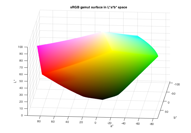
Here are another couple of view angles.

view(75,20)

view(185,15)

That's it for this week. Have fun with color-space surfaces!

Get the MATLAB code

Published with MATLAB® R2015a