Today I'll try to wrap up my discussion about how aliasing affects image resizing and about how the imresize function tries to prevent it. (This is called antialiasing.) Let me show you where we are going. Here is the zone plate image I showed last time.

Z = imzoneplate(501);
imshow(Z)
title('Z')

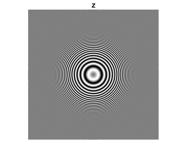
Here's what happens when we shrink Z by throwing away samples.

Z4 = Z(1:4:end,1:4:end);
imshow(Z4)
title('Z4')

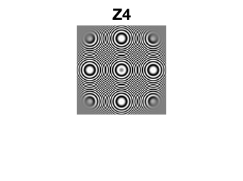
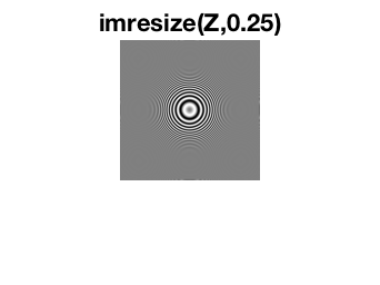
And here's what imresize does (with the default behavior):

Z4_imresize = imresize(Z,0.25);
imshow(Z4_imresize)
title('imresize(Z,0.25)')

Before I get started describing the imresize approach to antialiasing, I should say that there are several algorithm approaches to antialiasing in image resizing. This is just one. It is based on classical ideas from digital signal processing.

I'll use the notation that $f[n]$ is a function of a discrete variable $n$, and $f(x)$ is a function of a continuous variable $x$. Here's a way to think about the image resizing problem that is theoretically useful. To simplify the discussion for a bit, I'll talk in terms of 1-D signals. (Warning: people with a graduate-level background in digital signal processing will probably find this explanation too hand-wavy. Everybody else will find it too jargon-y. I'm doing my best.)

Suppose we want to convert a 1-D signal, $f[n]$, to another 1-D signal that has a different sampling rate.

There's a problem with the two-step procedure above. If the sampling rate for $g[n]$ is reduced from the original sampling rate of $f[n]$, then the procedure is susceptible to aliasing distortion if $f[n]$ contains high frequencies that cannot be represented at the lower sampling rate. To address this problem, let's insert another step in the procedure.

One key to understanding the imresize approach is to recognize that filtering with two filters in succession, in this case $h(x)$ and $h_a(x)$, can be replaced by one filter whose frequency response is the product of the original two filters. The second key to understanding the imresize algorithm is that the desired frequency response for the antialiasing filter, $h_a(x)$, depends how much we are changing the sampling rate. If we shrink the original signal more, then we have to remove more of the high frequencies with $h_a(x)$.

To state that more compactly (while waving my hands fairly vigorously), you can use just one continuous-domain filter to simultaneously accomplish interpolation and antialiasing.

Let me show you how this works for the cubic interpolation kernel that imresize uses by default. Here is the code for the cubic interpolation kernel:

function f = cubic(x)
% See Keys, "Cubic Convolution Interpolation for Digital Image
% Processing," IEEE Transactions on Acoustics, Speech, and Signal
% Processing, Vol. ASSP-29, No. 6, December 1981, p. 1155.

absx = abs(x);
absx2 = absx.^2;
absx3 = absx.^3;

f = (1.5*absx3 - 2.5*absx2 + 1) .* (absx <= 1) + ...
                (-0.5*absx3 + 2.5*absx2 - 4*absx + 2) .* ...
                ((1 < absx) & (absx <= 2));

(This code is inside the file imresize.m.) And here's what the interpolation kernel looks like:

figure
fplot(@cubic,[-2.5 2.5],'LineWidth',2.0)

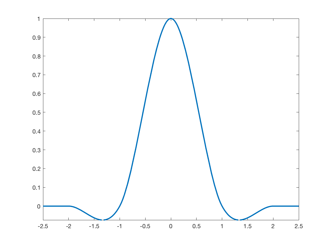
The function imresize then modifies the interpolation by stretching it out. The stretch factor depends directly how much we are shrinking the original signal. Here's the imresize code that modifies the interpolation kernel:

if (scale < 1) && (antialiasing)
    % Use a modified kernel to simultaneously interpolate and
    % antialias.
    h = @(x) scale * kernel(scale * x);
    kernel_width = kernel_width / scale;
else
    % No antialiasing; use unmodified kernel.
    h = kernel;
end

(I don't always comment my code well, but I think I did OK here.)

Notice that we don't modify the kernel at all when we are growing a signal (scale > 1) instead of shrinking it (scale < 1).

Here are three versions of the cubic interpolation kernel: the original one, one modified for shrinking by a factor of 2, and one modified by shrinking by a factor of 4.

h1 = @cubic;
h2 = @(x) 0.5 * h1(0.5*x);
h4 = @(x) 0.25 * h1(0.25*x);

fplot(h1,[-10 10],'LineWidth',2)
hold on
fplot(h2,[-10 10],'LineWidth',2)
fplot(h4,[-10 10],'LineWidth',2)
hold off

legend('h_1(x)','h_2(x)','h_4(x)')

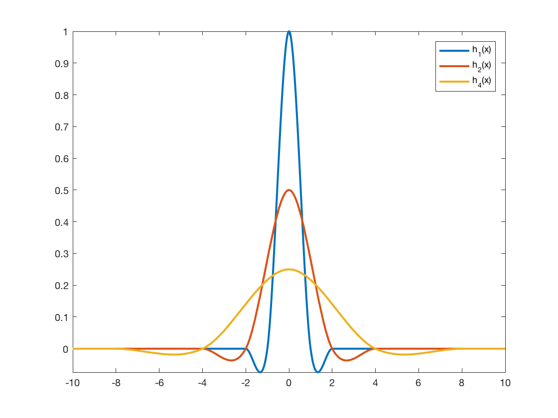
When we spread out the interpolation kernel in this way, the interpolation computation averages pixel values from a wider neighborhood to produce each output pixel. That is additional smoothing, which gives us the desired antialiasing effect.

Here is the imresize output for the zone plate image again.

imshow(Z4_imresize)

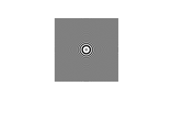
Only the rings near the center are visible. That's because those rings had lower spatial frequency in the original, and they can be successfully represented using only one-fourth the sampling rate. The higher-frequency rings further away from the center have been smoothed away into a solid gray.

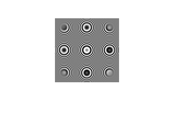
You can experiment yourself with imresize by disabling antialiasing. Here's how to shrink an image with antialiasing turned off:

Z4_imresize_noaa = imresize(Z,0.25,'Antialiasing',false);
imshow(Z4_imresize_noaa)

To give credit where credit is due, the algorithm used by imresize was inspired by the article "General Filtered Image Rescaling," by Dale Schumacher, in Graphics Gems III, Morgan Kaufmann, 1994.

Do you have other questions about imresize? Let me know by leaving a comment.

Get the MATLAB code

Published with MATLAB® R2016b