Aliasing and a sampled cosine signal
One challenge of teaching Fourier transform concepts is that each concept can be (and is) interpreted and explained in many different ways. It isn't always obvious how the different explanations for the same concepts are connected.
For example, in my last Fourier transform post I talked about aliasing. I said that if you sample a continuous-time cosine at a sampling frequency  , then you can't distinguish between a cosine with frequency
  and a cosine with frequency
  .
.
In response, Dave S. wanted to know how this related to what he learned about aliasing: that aliasing is a "problem that occurs when the sampling rate of your discrete signal is not at least twice the [...] highest existing frequency [in the continuous-time signal]."
I know I promised to introduce the discrete Fourier transform next, but I'd like to change my mind and try to answer Dave's question instead. There are two key pieces of the question to address: What is the nature of the "problem," and what is the significance of "twice the highest frequency"?
I thought about drawing some new frequency-domain diagrams showing overlapping triangles like you'd see in Oppenheim and Schafer, but then I thought it might be better to just continue the sampled cosine example from last time.
Let's start with a continuous-time cosine signal at 60 Hz.
f = 60;  % Hz
tmin = -0.05;
tmax = 0.05;
t = linspace(tmin, tmax, 400);
x_c = cos(2*pi*f * t);
plot(t,x_c)
xlabel('t (seconds)')
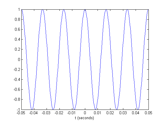
Let's sample  with a sampling frequency of 800 Hz.
T = 1/800;
nmin = ceil(tmin / T);
nmax = floor(tmax / T);
n = nmin:nmax;
x1 = cos(2*pi*f * n*T);
hold on
plot(n*T,x1,'.')
hold off
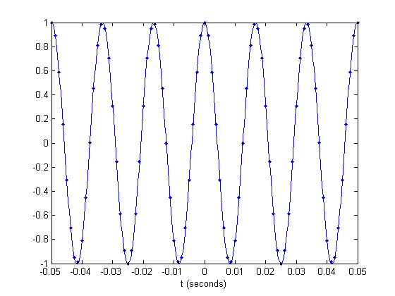
The sampling frequency of 800 Hz is well above 120 Hz, which is twice the frequency of the cosine. And you can see that the samples are clearly capturing the oscillation of the continuous-time cosine.
Let's try a lower sampling frequency.
T = 1/400;
nmin = ceil(tmin / T);
nmax = floor(tmax / T);
n = nmin:nmax;
x1 = cos(2*pi*f * n*T);
plot(t, x_c)
hold on
plot(n*T, x1, '.')
hold off
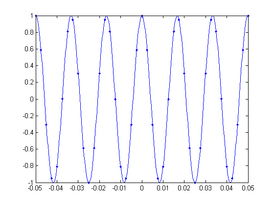
The samples above are still adequately capturing the shape of the cosine. Now let's drop the sampling frequency down to exactly 120 Hz, twice the frequency of the 60 Hz cosine. (And I'll switch to using circle markers to make the samples easier to see.)
T = 1/120;
nmin = ceil(tmin / T);
nmax = floor(tmax / T);
n = nmin:nmax;
x1 = cos(2*pi*f * n*T);
plot(t, x_c)
hold on
plot(n*T, x1, 'o')
hold off
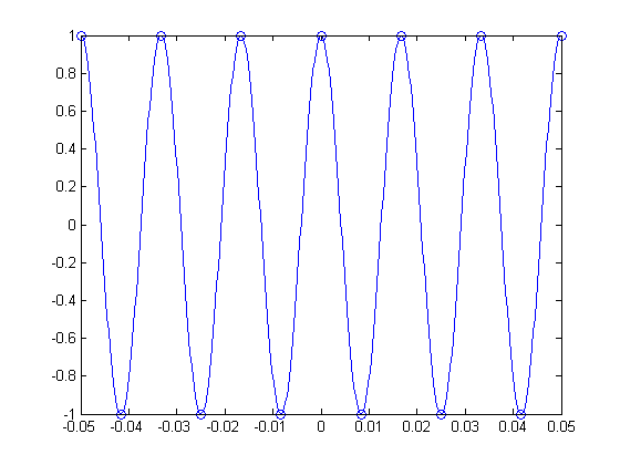
See how the samples jump back and forth between 1 and -1? And how they capture only the extremes of each period of the cosine oscillation? This is the significance of "twice the highest frequency of the signal" value for sampling frequency. If you'll allow a "hand-wavy" explanation here, I'll say that this sampling frequency of 120 Hz is just enough to capture the cosine oscillation.
But aliasing is worse that "just" losing information. When we drop the sampling frequency too low, the samples start to look increasingly like they came from a different, lower-frequency signal.
Let's try 70 Hz.
T = 1/70;
nmin = ceil(tmin / T);
nmax = floor(tmax / T);
n = nmin:nmax;
x1 = cos(2*pi*f * n*T);
plot(t, x_c)
hold on
plot(n*T, x1, 'o')
hold off
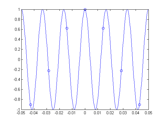
The samples above look like they actually could have come from a 10 Hz cosine signal, instead of a 60 Hz cosine signal. Take a look:
T = 1/70;
x_c = cos(2*pi*10 * t);
nmin = ceil(tmin / T);
nmax = floor(tmax / T);
n = nmin:nmax;
x1 = cos(2*pi*f * n*T);
plot(t, x_c)
hold on
plot(n*T, x1, 'o')
hold off
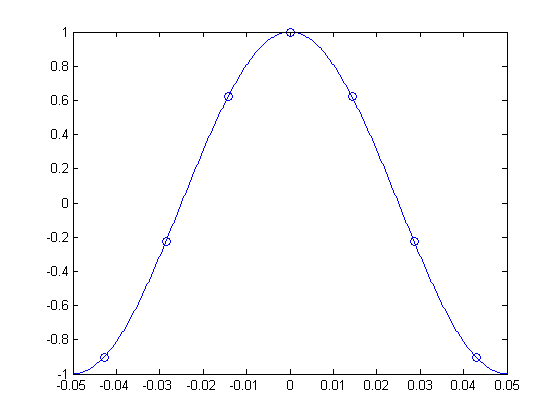
That's the heart of the "problem" of aliasing. Because the sampling frequency was too low, a high-frequency cosine looked like a low-frequency cosine after we sampled it.
Later on in this series I plan to come back again to the concept of aliasing and show some examples of how it looks in an image.
OK, now I'll start working on the upcoming discrete Fourier transform (DFT) post.
- Category:
- Fourier transforms




Comments
To leave a comment, please click here to sign in to your MathWorks Account or create a new one.